
search
0
All Posts By

Tim Kirschke

Tim Kirschke is a Managing BI Consultant and Head of Internal Development at Scalefree. With a background in Applied Mathematics, he specializes in architecting auditable data solutions using Microsoft Fabric, Snowflake, and dbt. A dbt Certified Architect and CDVP2, Tim has led major warehouse implementations and conducts strategic workshops on data automation and enablement.

Simplify Data Pipelines with Custom Macros in Coalesce.io

Custom Macros in Coalesce.io

When working in data transformation platforms like Coalesce.io, efficiency and maintainability are everything. As your data pipelines grow, so does the complexity of your transformation logic. This is where custom macros become a powerful ally — they let you write reusable, dynamic SQL code that can be applied consistently across your entire data model.

In this article, we’ll explore how to use macros in Coalesce.io with the help of the Jinja templating language. You’ll see how a small example — converting currency values from cents to dollars — can scale into a reusable pattern that saves hours of development and maintenance time.


What Are Macros in Coalesce.io?

Macros are reusable pieces of logic that can be dynamically inserted into your SQL transformations. They’re written in Jinja, a templating language originally popularized in web development frameworks such as Django and Flask. Coalesce.io leverages Jinja to make SQL more dynamic and parameterized, letting you write logic once and reuse it anywhere.

In simple terms, a macro is like a small function that can generate SQL code on the fly. You define a macro once — for example, to perform a mathematical conversion, a date calculation, or a string manipulation — and then call it across multiple nodes in your Coalesce.io project.

Why Use Macros?

As data models evolve, repetitive transformations become a maintenance challenge. Imagine you have multiple columns across different tables that need to be converted from cents to dollars. You could copy and paste the same transformation logic everywhere, but what happens when the business decides to change the precision or switch the data type?

You’d have to update every single instance manually — a process that’s time-consuming and error-prone. With a macro, you simply change the logic once, and it updates everywhere it’s used. This drastically reduces maintenance efforts and improves consistency.

Setting Up the Example: Converting Cents to Dollars

Let’s walk through a simple example. Suppose you have a customer table with an account_balance column that stores values in cents. The business requires all monetary values to be in dollars for reporting and analytics. This means we need to divide the column by 100 and adjust the data type accordingly.

In Coalesce.io, we can perform this transformation directly within a stage node. You might start with something like:

{{ SC }} / 100::NUMERIC(18, 2)

The {{ SC }} syntax tells Coalesce.io to dynamically insert the source column name. After running the transformation, you’ll see that account_balance is now expressed in dollars instead of cents. So far, so good — but what if multiple columns or nodes need this conversion?

Copying and pasting this logic everywhere quickly becomes inefficient. This is the perfect case for turning the transformation into a macro.

Creating a Custom Macro in Coalesce.io

To define a new macro, navigate to your project’s Build Settings and locate the Macros section. There, you can create workspace-level macros that are available across your entire Coalesce.io environment.

Here’s a simple Jinja macro to convert cents to dollars:

{% macro cents_to_dollars(column, scale=2) %}
    ({{ column }} / 100)::NUMERIC(18, {{ scale }})
{% endmacro %}

This macro does a few important things:

  • Accepts parameters — The column parameter specifies which column to transform, and scale defines the number of decimal places (defaulting to 2).
  • Performs the conversion — It divides the value by 100 and casts it to a numeric type.
  • Is reusable — You can now call this macro anywhere without rewriting the logic.

Applying the Macro in a Transformation

Once your macro is defined, you can use it directly within your stage or transform node. For example, if you want to create a new column that stores the converted dollar value, simply write:

{{ cents_to_dollars('customer.account_balance') }}

This will execute the macro, substitute the SQL expression, and generate the proper transformation logic dynamically. You can even adjust the precision if needed:

{{ cents_to_dollars('customer.account_balance', scale=4) }}

With just one line of code, you’ve achieved a flexible, reusable transformation that can be applied across multiple nodes and columns.

Benefits of Using Macros in Coalesce.io

Macros may seem like a small feature, but their impact on data engineering workflows is significant. Here are a few key advantages:

1. Reduce Maintenance Overhead

When transformation logic changes, you only need to update it in one place. This ensures consistency across your pipelines and minimizes human error.

2. Promote Reusability

Macros make your codebase more modular. Teams can share standardized transformation logic, reducing duplication and ensuring best practices are applied everywhere.

3. Improve Readability

Instead of cluttering transformations with complex SQL expressions, you can reference clean, descriptive macro calls. This improves readability and helps onboard new team members faster.

4. Enhance Collaboration

Macros can be shared across teams or workspaces, enabling collaborative development in larger analytics engineering environments.

5. Simplify Complex Logic

As transformations get more sophisticated, you can encapsulate multi-step logic inside a macro. For example, handling data type conversions, conditional mappings, or even custom business rules — all within one reusable function.

Debugging and Testing Macros

Because macros generate SQL dynamically, debugging can sometimes feel tricky. Coalesce.io helps by allowing you to preview the compiled SQL code. After running a transformation that uses a macro, open the results to view the underlying SQL — you’ll see exactly how your macro was expanded and executed.

This visibility is crucial for validating logic and ensuring your macros behave as expected.

When to Use Macros

A good rule of thumb is simple:

If you find yourself repeating the same transformation in more than one place, consider turning it into a macro.

Macros are particularly useful for:

  • Currency or unit conversions
  • Data cleansing logic (e.g., trimming whitespace, normalizing case)
  • Timestamp or date formatting
  • Standard calculations (e.g., margin, growth rate, ratios)
  • Conditional logic applied across multiple datasets

By standardizing these repetitive transformations, your data environment becomes cleaner, easier to manage, and more scalable.

Best Practices for Writing Coalesce.io Macros

  • Keep macros simple — Each macro should serve a single clear purpose. Break complex logic into smaller, composable macros when possible.
  • Use default parameters wisely — Providing defaults (like scale=2) makes macros flexible and user-friendly.
  • Document your macros — Add comments explaining what each macro does and the parameters it expects. Future maintainers will thank you.
  • Test before scaling — Validate each macro on a small dataset before applying it widely.
  • Version control your macros — Store them in a shared Git repository or Coalesce.io workspace for collaboration and traceability.

Real-World Impact

In production environments, macros can save hours of repetitive work each week. Imagine applying the same data type conversion or formatting rule across dozens of tables — a single macro call replaces all those redundant SQL snippets.

Macros also make large-scale refactoring much safer. If a business requirement changes (for example, moving from numeric to money data types), one macro edit automatically updates every transformation that depends on it.

Final Thoughts

Custom macros in Coalesce.io aren’t just a convenience — they’re a foundation for scalable, maintainable data engineering. By abstracting common logic into reusable templates, you streamline your transformations, reduce technical debt, and empower your team to focus on building insights rather than maintaining code.

As a best practice, always look for opportunities to generalize repetitive logic. When you spot patterns across transformations, that’s your cue to create a macro. Start small, experiment, and watch your data pipelines become cleaner, faster, and easier to manage.

Next Steps

Explore Coalesce’s documentation on macros and Jinja templating to deepen your understanding. You can also download our free Data World Handbook — a comprehensive guide to modern data architecture, data vault modeling, and transformation best practices.

And if you’ve built interesting macros of your own, share them in the comments below. We’d love to see how you’re simplifying your Coalesce.io workflows.
Watch the Video

Monitoring of a Snowflake Powered EDW

Snowflake Built-In Tools

Introduction to Snowflake

Snowflake established itself as one of the most widely used cloud data platforms, providing a scalable and flexible architecture for building, maintaining, and operating Enterprise Data Warehouses. While it aims to eliminate data silos and simplify the data structure, with billions of queries a day (overall), its elastic computing handles the workload for good performance and a satisfied customer.

However, as organizations rely increasingly on Snowflake, monitoring their solution might be crucial for performance optimization, error and root cause analysis, and cost control. Although Snowflake handles these tasks very well on its own, experience shows some need for human interference when it comes to more complex queries, to increase performance, lowering the runtime without upscaling or scaling out.

This blog article aims to provide general information about and technical insights into Snowflake. Focusing on techniques as well as built-in tools to analyze bottlenecks, we aim to potentially increase performance and therefore decrease unnecessary costs.


Snowflake Built-In Tools

Query History

Starting with Snowflake’s built-in tools, we will dive into its roots and combinations of several metrics.

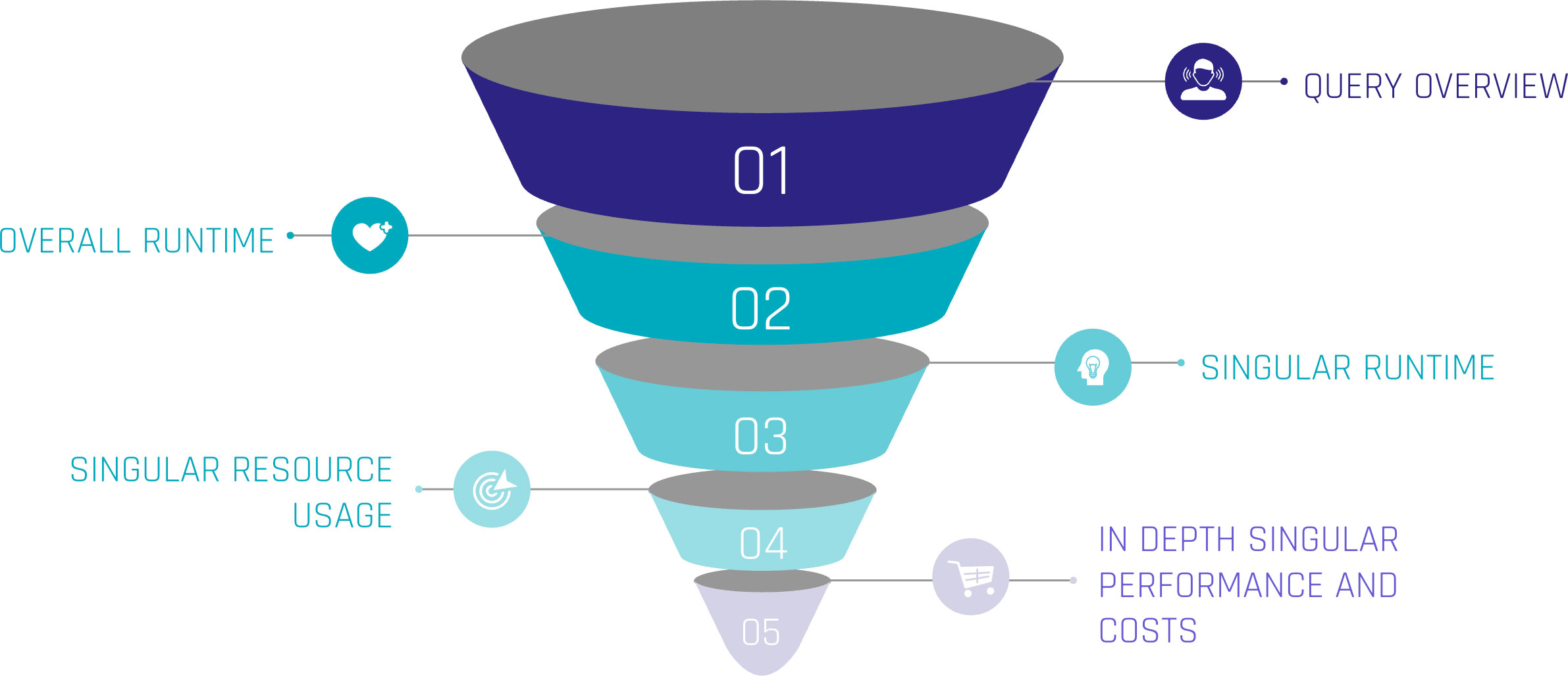
Monitoring query performance includes several depths of insight, from an overview of the general query history, down to the performance of each individual step within a query.

Snowflake Built-In Tools

Let’s assume the top level as an overview of our queries. Including metrics such as:

  • Start Time,
  • Total Time,
  • Status and
  • Query Type.

For the first level, we can gain insights when the queries start, how much time they were consuming, whether they succeeded or failed, or even are still running. Lastly, we can see the type of query, such as ‘CREATE TABLE’, ‘INSERT’, or ‘SELECT’. At this level, a brief overview could be created about the traffic within the Warehouse.

When hearing about this, you may be familiar with a built-in tool called ‘Query History’, which tracks this kind of information automatically without the need for user interference. It is easily available within the sections ‘Monitoring’ and ‘Query History’.

Query Profile

Further, it is easily possible to extract more information about the executed queries. Every single query within the ‘Query History’ has a unique identifier and attached metrics. Within the ‘Query History’ section, when choosing a query by simply clicking on it, we gain insights into the single query. These include two main sections.

‘Query Details’ delivers information about the query in general. Including the above-mentioned ‘Start Time’, ‘End Time’, ‘Warehouse Size’, and ‘Duration’, which is divided into ‘Compilation’, ‘Execution’, and further time-consuming steps.

‘Query Profile’ describes the execution plan of the query as a graphical representation. Each step within the query, such as ‘SELECT’, ‘JOIN’, and ‘WHERE CONDITION’ are represented as nodes within the graph. These nodes are operations, triggered by the query. Each fulfilling a task like filtering data, selecting data rows, but also scanning results, and reading data from cache. Snowflake interprets the written SQL and creates a performant execution plan by itself.

Despite that, each node consumes more or less resources, depending on the SQL code itself, the underlying dataset, and the Warehouse configurations. Using the ‘Query Profile’, we can identify the most time-consuming steps in our query, such as false ‘JOINS’, and work around those nodes to identify more performant solutions. Therefore, the ‘Query Profile’ provides detailed information about each node, like processing time, cache scanning, and partition pruning. For further information, check out the Snowflake Documentation.

Custom Monitoring Solution

But when Snowflake already provides a solution, why do we need separate monitoring?

Although already delivered, your requirements may vary from the existing solution. With the built-in tools mentioned above, the possibility to check on each query is given. Additionally, Snowflake may not be the only tool used for data processing. ELT tools like dbt or Coalesce help data engineers improve processes. To include these further metrics from outside Snowflake, a custom monitoring solution, based on Snowflake’s delivered metrics, is needed.

With this in mind, the following section focuses on our own scalable monitoring solution.

Account Usage and Information Schema

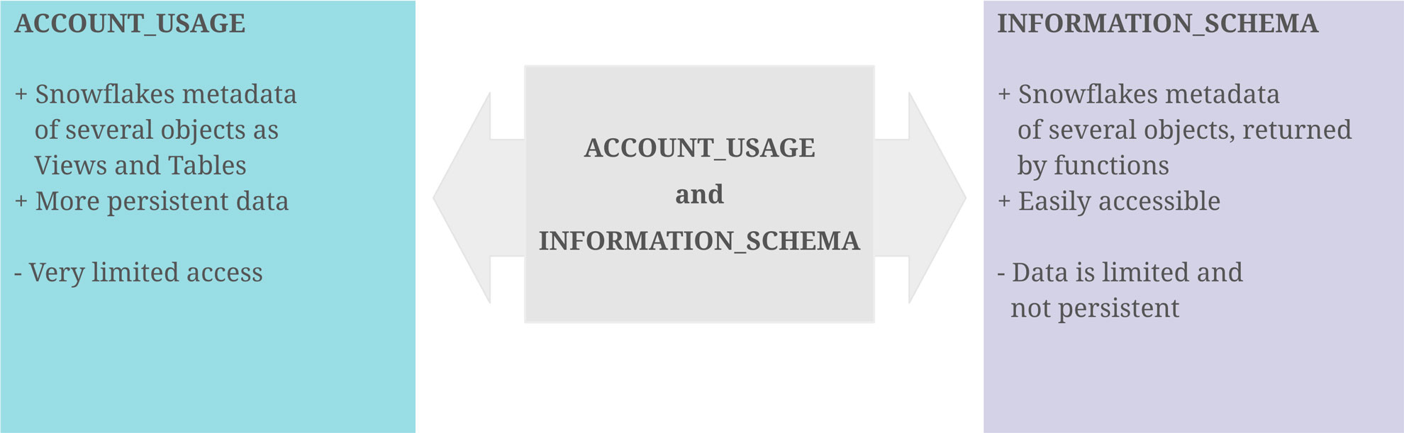
With the idea that the data of the graphical output exists as a table or view, containing all data necessary, it turns out that Snowflake provides us the schemas ‘ACCOUNT_USAGE’ and ‘INFORMATION_SCHEMA’, fulfilling this purpose. They provide similar opportunities for this challenge, although there are some differences.

‘ACCOUNT_USAGE’ provides insights into Snowflake metadata of several objects. This includes ‘QUERY_HISTORY’, which contains the information described in the sections above. The query history is available for all queries within the last 365 days. This enables the loading of metrics entities in the Data Warehouse, making the information readily accessible and persistent for daily, weekly, or monthly processes. The downside is that access to the ‘ACCOUNT_USAGE’ schema is often limited.

The ‘INFORMATION_SCHEMA’ contains a set of system-defined views and tables, providing metadata and information about created objects. Using predefined functions on the ‘INFORMATION_SCHEMA’, metadata can be retrieved, which, on the other hand, is limited to some factors. As this option is more accessible for developers, the focus remains on this option.

Account Usage and Information Schema

Extract Metrics Data

At the beginning, it is crucial to point out the limitations and possibilities of this approach. For the scope of this blog, two functions on the ‘INFORMATION_SCHEMA’ are needed.

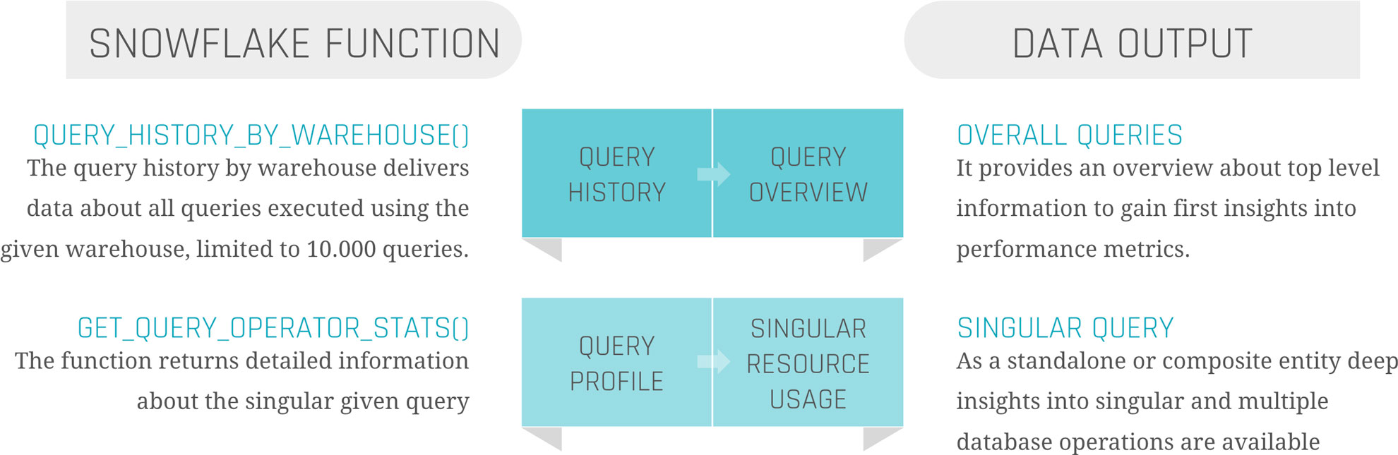
‘QUERY_HISTORY_BY_WAREHOUSE()’ is equal to ‘QUERY_HISTORY’.

‘GET_QUERY_OPERATOR_STATS()’ is the equivalent of ‘QUERY_PROFILE’.

‘QUERY_HISTORY_BY_WAREHOUSE()’ takes four different arguments.

  • ‘WAREHOUSE_NAME’ – The name of the Warehouse executing the queries
  • ‘END_TIME_RANGE_START’ – Time range within the last 7 days, in which the query started running
  • ‘END_TIME_RANGE_END’ – Time range within the last 7 days, in which the query completed running
  • ‘RESULT_LIMIT’ – The number of the maximum returned rows. The default lies by ‘100’, the range by ‘1’ to ‘10.000’

The output is the ‘QUERY_HISTORY’ as a structured table with some extra information. Each query is displayed in one row. Therefore, the metrics are aggregated into one specific query.

The most critical limitation seen here is the ‘RESULT_LIMIT’ and ‘END_TIME_RANGE_*’, as it forces us to retrieve the data before the 7-day retention ends and before 10.000 other queries have been executed. Depending on the size of the Warehouse and the scope of the monitoring range, the extract and load process must be customized.

‘GET_QUERY_OPERATOR_STATS()’ takes one argument.

  • ‘QUERY_ID’ – The unique ID of the executed query.

The output is a structured table of the ‘QUERY_PROFILE’ of one specific query. Each step in the execution plan is displayed as one row, so the output size depends on the complexity of the query itself. Each node is detailed with available metadata, breaking down information from ‘GET_QUERY_OPERATOR_STATS()’ into individual steps. This allows for a deeper analysis of performance metrics, helping to identify any bottlenecks.

As the function is on query-level, it is not done by joining the table outputs of those two functions together to get a satisfactory result. Further steps are needed.

Load Metrics Data

Load Metrics Data

Before filtering, transforming, or joining the data, it is suggested to load the data as it comes into persistent tables.

Snowflake Query History

The first step should be to create the table when calling the function, already combining these two components to avoid missing capture data, columns, or false data types. To keep continuous loading, use your preferred ELT tool to append the process at the end, or set up a scheduled Snowflake Task, considering the limitations mentioned above.

Snowflake Query Profile

This process is more complex. To load the data, it is not sufficient to simply call the function once for the query history. To ensure data integrity and a clear 1:n solution (1 row in the query history, n>0 rows in the query profile), it is needed to iterate through the list of all query IDs inside the query history and run the function for each one of them. Each of the resulting datasets needs to be inserted into the corresponding table.

Information Delivery

Now, as the data is extracted and loaded, the last remaining steps are transforming the data and information delivery. As this strongly depends on the use case, we focus on linking the two metrics tables and creating a standard dashboard inside Snowflake to show the results.

Our two tables ‘snowflake_query_history’ and ‘snowflake_query_profile’ are in a soft relation, where the “QUERY_ID” serves as a unique identifier to link each query from the query history to its query profile. Therefore, joining both tables on the “QUERY_ID” is indispensable. The first decision to be made is whether to keep one row for each query and aggregate the object constructs or to split it up into its individual steps, like within the query profile. For simplicity, we focus on the second option to avoid complex SQL statements for the dashboard. As the SQL statement only includes the ‘SELECT’ and ‘JOIN’ operators, you may choose a view as materialization, instead of a table.

With the possibility of creating dashboards out of Snowflake worksheets, it is relatively easy to integrate simple SQL statements into the dashboard, represented as charts. For some examples, we will take a look at the resulting data.

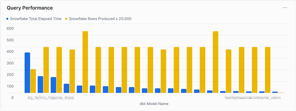
Query Performance

This example shows the top 20 queries by ‘TOTAL_ELAPSED_TIME’, the overall time the query needs to compile, run, waiting time, and other technical steps. As noticed by the chosen x-axis label, Snowflake’s metrics can be combined using other tools, such as dbt. It is set to compare this time against the produced rows to gain some insights into whether the queries can handle much data or not. As can be seen, the query consuming the most time, and therefore credits, does not produce the most rows. At this point, we may be interested in gaining some insights into the query itself.

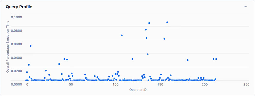
Query Profile

Showing each Operator with its corresponding relative runtime, only a handful exceed 5% of the total execution time. This may indicate that within the SQL statement, only a few steps need to be optimized to create an overall more performant query.

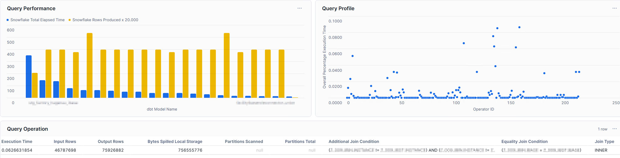
Query Dashboard

With this in mind, the single query can also be analyzed in the dashboard. For example, you may take into account input rows and output rows, bytes spilled, partitions scanned, and partitions total, or the join condition. Furthermore, you may not only gain insights into your query performance, but also into your table management, such as clustering and partitioning. Additionally, you are also capable of integrating more metrics coming from external sources and linking them directly to Snowflake, making it a powerful monitoring solution.

Conclusion

Snowflake offers a powerful and highly adaptable cloud data platform that meets the demands of modern enterprise data warehousing. However, as data volume and complexity grow, so does the need for proactive monitoring and optimization to ensure continued performance and cost efficiency. By leveraging Snowflake’s built-in tools and implementing strategic performance-enhancing techniques, organizations can address bottlenecks effectively and optimize query performance.

In this article, we addressed the opportunities given through Snowflake’s built-in tools and how to effectively use them. We learned that although these tools are great, to gain a fast and high-level overview, as well as detailed insights at the same time, it is relatively easy to create your own dashboard with the loaded data. Therefore, you are able to analyze and evaluate it, as well as make optimum use of resources to enable high-performance operation without increasing cost by scaling up or scaling out.

Creating Data Vault Links with Coalesce.io

Data Vault Links

Data Vault modeling separates data into hubs, links, and satellites to support scalable, auditable, and historized data warehouses. Links represent relationships between business entities (hubs) — for example, which supplier delivers which part. Coalesce.io makes creating Data Vault objects fast by providing a GUI-driven workflow for building stages, generating hash keys, and creating links that can be run incrementally against a target like Snowflake.

This article walks through the exact process demonstrated in the video transcript: exploring source tables, creating a Data Vault stage, generating hash columns, building a single-source link, then extending it to a multi-source link. The goal is to give you a clear checklist and practical tips so you can reproduce the steps in your Coalesce.io environment.


Why create a Data Vault link?

In Data Vault, links are the canonical way to model relationships between business entities. A link contains:

  • a link hash key — generated from the business keys of all participants
  • the hub hash keys of every participating hub
  • load metadata such as load timestamp and record source

Creating links gives you an integrated relational layer independent of the transactional sources. Links allow you to track relationship history and stitch together hubs for downstream analytics and satellites.

Overview of the source data used

In the example from the video, you start with two resource tables in Coalesce:

  • parts — defines parts with attributes like brand, name, type, size, and contains a reference to a supplier.
  • suppliers — contains supplier metadata and a supplier key.

The parts table contains a column that references the supplier key, so semantically there is a relationship: part → supplier. This is the relationship we model as a Data Vault link.

Step 1 — Create a Data Vault stage in Coalesce

Every Data Vault object creation in Coalesce.io should start from a Data Vault stage. The stage is where you prepare the source rowset and add the derived columns that your downstream hub/link/satellite will need (hash keys, record source, load date, etc.).

  1. Right-click the source entity (in the video: parts) and select Node → Data Vault for Coalesce → Stage.
  2. Coalesce.io creates a new object (e.g., DV_stage_parts) and forwards the source columns into the stage.
  3. Add any extra columns you need for the link: a hash key for the part hub, a hash key for the supplier hub, and the combined link hash key.

Best practice: keep the naming consistent. If the column will become the hub hash key for part, name it something like HK_part_H. That makes it obvious where the column flows later.

Step 2 — Generate hub hash keys and the link hash key

Hash keys are central to Data Vault 2.0 implementations. They provide stable, compact identifiers for business keys and are typically generated using a deterministic hash function (often MD5 or SHA). In Coalesce.io you can generate these with the GUI.

  1. Right-click the business key column for the part and choose Generate hash column — rename it to HK_part_H.
  2. Repeat for the supplier business key and call it HK_supplier_H.
  3. Select both business key columns (or both generated hash columns) and choose Generate hash column again to produce the link hash. Name it something descriptive, like HK_part_supplier_L (L for link).

Important: the link hash must be calculated from the business keys (or their hub hashes) of all relationship participants and in a deterministic order. That ensures the same relationship always produces the same link hash across sources and loads.

Step 3 — Select only the columns you need for the link

Coalesce.io lets you choose which stage columns flow into the next object. For the link you typically need:

  • the link hash key (first column)
  • the hub hash keys for all participants (in order)
  • load metadata: LoadDate or LoadId, and RecordSource

Select these five (or more if you want custom metadata) and then create the Data Vault link node by right-clicking → Node → Data Vault for Coalesce → Link.

Step 4 — Configure the link object

When the new link object appears, follow these checks:

  • Confirm the link hash column is the first column and matches your naming standard (e.g., HK_part_supplier_L).
  • Verify the hub hash keys follow — HK_part_H then HK_supplier_H.
  • Make sure load metadata (load timestamp/id and record source) are present.
  • Open the Data Vault options panel in Coalesce.io and explicitly set which column is the link hash. This tells the Coalesce.io macro how to populate the link.

Click Create and then Run. Coalesce.io will generate and execute an INSERT statement (an incremental load) against your target (Snowflake in the example).

Tip: check the generated SQL before running. Coalesce.io usually issues an incremental INSERT that only adds new link rows, so the second run often returns “0 rows inserted” when there are no new relationships — that’s expected and desirable.

Step 5 — Inspect results and generated code

After running, Coalesce.io shows the result set and the generated SQL. In the video, the first execution inserted the bulk of rows (e.g., hundreds of thousands), and subsequent runs inserted zero because no new relationships existed. This shows the incremental behavior is functioning correctly.


-- example pseudo-SQL generated by Coalesce
INSERT INTO dv_link_part_supplier (...)
SELECT ...
FROM staging.dv_stage_parts
WHERE NOT EXISTS (
SELECT 1 FROM dv_link_part_supplier l
WHERE l.hk_link = staging.hk_part_supplier_l
);

Always validate the counts and confirm that the link hash values are unique per relationship. If you see duplicates or mismatches, re-check the hash generation order and the columns used.

Creating a multi-source link

A common Data Vault case is that the same relationship may appear in multiple source systems (e.g., ERP, procurement feed, third-party data). Data Vault links are designed to aggregate relationship evidence across sources. Coalesce.io supports multi-source links by allowing you to add additional source mappings to the link object.

The workflow from the video:

  1. Create or update a stage for the second (or additional) source that produces the same five columns (link hash, hub hashes, load metadata).
  2. On the link object in Coalesce, open the multi-source mappings and add a new source mapping (e.g., part_sub_source).
  3. Map the source stage columns to the link columns — Coalesce.io often auto-maps if names match.
  4. Run the link. Coalesce.io will process both sources and insert any newly observed relationships.

Note: If you run into an error where Coalesce.io cannot find the link hash for the new source, make sure the stage includes the generated join or column you intended to hash. In the video, the speaker realized they needed to explicitly build the join in the stage (generate the joined dataset) before the link could reference its hash column.

Common pitfalls & best practices

  • Hash ordering: Always use a consistent ordering for participants when generating the link hash (e.g., alphabetical by object name or a documented canonical order).
  • Naming conventions: Adopt a clear naming convention: HK_<object>_H for hub hashes and HK_<a>_<b>_L for link hashes. Consistency helps Coalesce.io auto-map and keeps downstream ETL predictable.
  • Stage first: Always prepare your stage before creating a link. The stage is where joins, derived fields, and hash generation happen.
  • Record source & load metadata: Always include record source and a load timestamp or load ID in the link so you can trace where and when a relationship was observed.
  • Incremental testing: Run the insert once to ingest the historical baseline, then run it again to verify zero rows are inserted when no changes exist.
  • Multi-source growth: Plan for adding multiple sources over time — links should be able to accept additional source mappings without rework.

When to add satellites

Links can also have satellites if you want to capture attributes specific to the relationship (for example, contract terms, effective dates, or relationship status). If you need to historize relationship attributes, create a satellite for the link and drive it with a hash diff or change detection strategy.

The video skipped satellite configuration because its focus was link creation, but be mindful that links + satellites are the full pattern for historized relationship data in Data Vault.

Conclusion

Creating Data Vault links with Coalesce.io is a straightforward, GUI-assisted process once you follow a repeatable pattern:

  1. Create a Data Vault stage for your source rows.
  2. Generate hub hash keys for all participating entities.
  3. Generate a deterministic link hash from the participants’ business keys (or hub hashes).
  4. Select the required columns and create the link object.
  5. Configure multi-source mappings as needed and run incremental loads.

Following these steps ensures your links are consistent, auditable, and ready for enterprise-grade analytics. If you haven’t implemented hubs yet, consider building hubs first (or in parallel) so your link hub keys map cleanly into the rest of the Data Vault model.

Happy modeling — and if you’re using Snowflake as your target, double-check the generated SQL from Coalesce.io and watch the run results to validate incremental behavior.

Watch the Video

Databricks and dbt: A Practical Approach to Data Vault Implementation

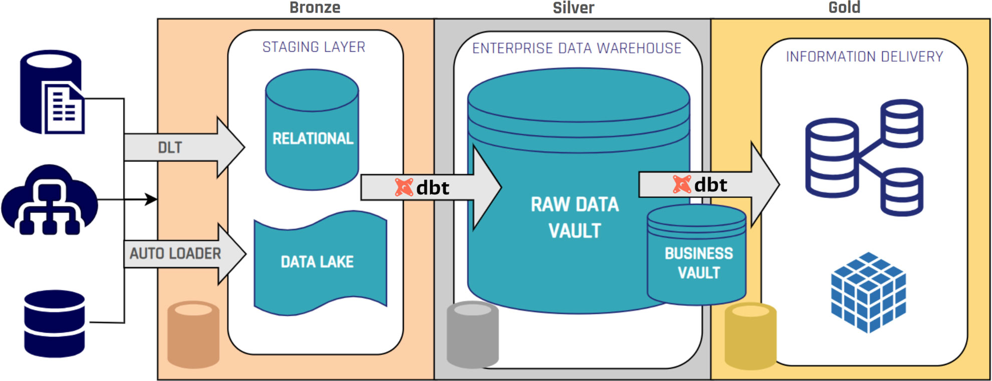
Bronze Silver and Gold layers in the Data Vault Structure

Databricks and dbt

Selecting the appropriate technology stack is a critical factor in the successful delivery of a Data Vault 2 architecture. Two technologies that work effectively together at a large scale data solutions are Databricks and dbt. When combined, they provide a practical way to implement Data Vault models while addressing performance, governance, and auditability requirements.

It can be argued that dbt’s role in a Databricks-based architecture is not always essential, since many of its core capabilities (such as transformation scheduling, lineage tracking, and documentation) can also be implemented using native Databricks features. Understanding the specific role each tool plays helps clarify where they complement each other and where functionality overlaps.


Databricks as the Processing and Storage Platform

Databricks’ Lakehouse architecture combines the scalability of a data lake with the reliability of a warehouse. Its Delta Lake technology offers ACID transactions, schema enforcement, and time travel, enabling precise historical querying, which are relevant aspects when it comes to Data Vault’s historization requirements.

With Unity Catalog, Databricks centralizes metadata management and enforces fine-grained access control, ensuring sensitive attributes are protected without introducing unnecessary satellite splits. This alignment between governance and performance is particularly relevant in Data Vault environments.

dbt as the Transformation and Orchestration Layer

dbt manages and automates SQL-based transformations in a modular and version-controlled manner. In a Data Vault context, dbt enables:

  • The creation of Hubs, Links, and Satellites through templated, reusable models. Here, different packages can be leveraged, like our datavault4dbt package, which is constantly updated to be fully compliant with the most recent Data Vault standards.
  • Integrated testing to validate business keys, relationships, and data quality.
  • Automated documentation that directly reflects the structure and dependencies of the Data Vault.

This structured approach makes transformations transparent and repeatable, supporting the auditability requirements inherent to Data Vault.

Integration in a Data Vault Workflow

When Databricks and dbt are deployed together:

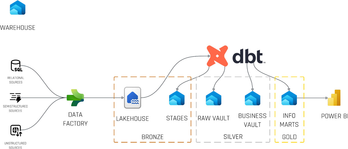
  • Data ingestion occurs in Databricks, storing raw datasets as Delta tables, usually in the Bronze layer.
  • dbt transformations generate Raw Vault entities and Business Vault objects in the Silver layer.
  • Governance and security controls are enforced via Unity Catalog without altering the Data Vault model structure.
Bronze Silver and Gold layers in the Data Vault Structure

This approach preserves Data Vault’s methodological structure while using Databricks’ distributed compute and storage capabilities.

Business Value when combining dbt and Databricks

The combined use of Databricks and dbt offers:

  • Scalable processing of large, complex datasets: Databricks handles enterprise-scale data efficiently, while dbt structures transformations into modular, reusable components.
  • Consistent governance across all layers of the Data Vault: dbt’s lineage and documentation, plus Unity Catalog’s access control, ensure compliance and transparency end to end.
  • Lower operational risk through tested, version-controlled transformations: Git-based versioning and automated tests in dbt reduce errors before execution on Databricks.
  • Improved query performance for information marts and analytics: Delta Lake optimizations and dbt’s pre-aggregated tables with business logic minimize expensive joins.

For organizations building Data Vault on Databricks, dbt strengthens structure and quality while Databricks ensures scalability and performance.

Get Started with dbt: A Quick 15-Minute Guide Using Snowflake

Get Started with dbt Using Snowflake

Introduction to dbt

dbt (data build tool) revolutionizes the way teams build and maintain analytics workflows by bringing software‐engineering best practices to SQL‐based data transformations. Instead of ad‐hoc scripts, dbt encourages version control, modular models, testing, documentation, and lineage graphs. In this guide, you’ll learn how to go from zero to your first dbt models—running entirely in the cloud on Snowflake—in under 15 minutes.


Why Choose dbt Cloud + Snowflake?

  • Fully managed: No local install or complex orchestration; dbt Cloud handles hosting.
  • Quick setup: Snowflake’s partner connector spins up a dbt trial, pre-configured with your credentials.
  • Best practices out of the box: Built-in IDE, job scheduling, Git integration, and documentation.
  • Scalable performance: Leverages Snowflake’s compute power for fast model builds.

Prerequisites

  1. A Snowflake trial account (free, 1-minute setup).
  2. A modern browser (Chrome, Firefox) or VS Code for remote development.
  3. Basic familiarity with SQL.

1. Launching dbt Cloud from Snowflake

Once logged into your Snowflake trial, navigate to the Data Products → Partners → Connect pane. Scroll to find the dbt entry and click Connect → Launch. This will automatically:

  • Provision a dbt Cloud trial account
  • Create a new Snowflake database and warehouse
  • Inject Snowflake credentials into your dbt Cloud connection

You’ll land in the dbt Cloud dashboard, ready to start your first project.

2. Exploring the dbt Cloud UI

In dbt Cloud’s left navigation bar you’ll find:

  • Develop: Interactive IDE for coding models, sources, tests, documentation.
  • Deploy: Job definitions, environments, and run history.
  • Documentation: Auto‐generated docs site with lineage graphs.
  • Settings: Account, project, and Git integration.

Click Develop → IDE (hosted in Chrome or connect your VS Code). Let’s initialize our dbt project.

3. Initializing Your dbt Project

  1. In the IDE, open the Version Control pane and click Initialize dbt Project.
  2. Accept the defaults; dbt creates a dbt_project.yml and folder structure (models/, macros/, etc.).
  3. Commit the auto‐generated files in a new Git branch: “initialized dbt project”.

Your Git pane now shows uncommitted files; click Commit & Push to save the project baseline.

4. Defining Your Source Data

dbt doesn’t load data from external systems—you must point it to existing tables. Snowflake’s sample database (SNOWFLAKE_SAMPLE_DATA) contains TPC-H tables you can use.

Create a new YAML file under models/ named sources.yml with:

version: 2

sources:
  - name: tpch
    database: SNOWFLAKE_SAMPLE_DATA
    schema: TPCH_SF1
    tables:
      - name: CUSTOMER
      - name: ORDERS

Save to see the lineage graph update with two new source nodes.

5. Building a Staging Model

Staging models standardize raw tables and prepare them for downstream transformations. In models/, delete the example/ folder and instead:

  1. Create a folder called models/staging/tpch.
  2. In that folder, create stg_tpch_customer.sql:
{{ config(materialized='view') }}

select
  C_CUSTKEY   as customer_key,
  C_NAME      as customer_name,
  C_ACCTBAL   as account_balance,
  C_COMMENT   as comment
from {{ source('tpch', 'CUSTOMER') }}

Notes:

  • The source() macro resolves to the fully qualified table.
  • materialized='view' tells dbt to build a view by default.

Save and click Run → dbt run to build just this model. In seconds you’ll see a view in your Snowflake UI under the dev schema.

6. Creating a Production-Ready Dimension

Dimensions (Gold layer) contain curated, business-ready tables. Let’s filter for customers with positive balances.

  1. Create models/marts/customer_dim.sql:
{{ config(materialized='table') }}

select
  customer_key,
  customer_name,
  account_balance
from {{ ref('stg_tpch_customer') }}
where account_balance > 0

Here, ref() links to another model, ensuring correct build order and clear lineage.

Click Compile to preview generated SQL, then Run → dbt run to create the table in Snowflake.

7. Testing and Documentation

dbt encourages tests to enforce data quality:

  • Add to models/staging/tpch/schema.yml:
version: 2

models:
  - name: stg_tpch_customer
    tests:
      - not_null:
          column_name: customer_key
      - unique:
          column_name: customer_key

Run dbt test to validate your models. Any failures will be reported in the UI.

Generate documentation with dbt docs generate, then preview via dbt docs serve. Explore your project’s lineage graph and column descriptions.

8. Version Control & Deployment

dbt Cloud integrates Git for collaboration. After feature development:

  1. Commit your branch and open a pull request (GitHub, GitLab, Bitbucket).
  2. Merge into main.

In Deploy → Environments, create a production environment. Under Jobs, define a job that runs:

  • dbt seed (if you have local CSV seeds)
  • dbt run
  • dbt test

Schedule the job (e.g., hourly, daily) or trigger it on Git commits. Monitor run history and logs directly in dbt Cloud.

9. Best Practices & Next Steps

  • Modularize models: Break complex logic into smaller models.
  • Document extensively: Use YAML descriptions for sources, models, and columns.
  • Implement CI/CD: Integrate dbt Cloud jobs with your team’s CI pipeline.
  • Leverage analyses: Create analyses/ for ad-hoc queries and charts.
  • Scale with packages: Reuse community packages (e.g., dbt_utils).

For deeper dives, explore the official dbt documentation and the dbt Hub for community packages and best practices.

Watch the Video

Conclusion

In just a few steps, you’ve:

  • Provisioned dbt Cloud via Snowflake
  • Initialized a dbt project with Git
  • Defined raw sources and built staging models
  • Created a production dimension with ref()
  • Tested data quality and generated documentation
  • Set up a CI/CD job for automated deployment

Now you have a repeatable, maintainable analytics pipeline. Keep building new models, add tests, and document as you go—your future self (and team!) will thank you.

Leveraging the Coalesce API: A Practical Guide for Data Engineers

About the Coalesce API

In today’s fast-paced data-driven world, automation, integration, and scalability are crucial for modern data engineering. The Coalesce API empowers developers, analysts, and engineers to streamline their workflows, integrate with external tools, and build robust data pipelines. Whether you’re migrating data, monitoring runs, or embedding data tasks into your existing scheduling systems, the Coalesce API offers the flexibility and power you need.

This guide will walk you through the Coalesce API’s key features, show you how to get started, and explore real-world use cases that can elevate your data operations.


API Features

The Coalesce API is structured into two primary segments: the Coalesce API itself and the Run API. Each provides a specific set of endpoints designed to help you interact programmatically with the coalesce.io platform.

Coalesce API Endpoints

  • Get / List Environments: Fetch available environments where your coalesce.io projects live.
  • List / Get / Create / Set Nodes: Manage your data transformation nodes—essential building blocks of any pipeline.
  • List / Get Runs: Retrieve historical or current run information for traceability and auditing.
  • List Run Results: Analyze outputs and diagnostics of your executed runs.

Run API Endpoints

  • Start / Stop / Retry Run: Full control over triggering, halting, or retrying your pipeline executions.
  • Check Live Run Status: Monitor real-time status of ongoing processes.

These features provide a comprehensive toolkit for orchestrating and managing your Coalesce-powered data architecture.

Using the API

One of the strengths of the Coalesce API is its accessibility across a wide range of tools and platforms. Here’s how you can explore and interact with the API in your development environment:

  • API Explorer: Use the built-in API Explorer for hands-on experimentation and learning.
  • Postman Collection: Easily import the Coalesce API into Postman to structure and test API calls efficiently.
  • Insomnia: Another popular REST client for interacting with coalesce.io endpoints with ease.
  • Command Line: cURL and other CLI tools allow direct HTTP requests for automation and scripting.
  • Azure Data Factory: Seamlessly integrate coalesce.io into your Azure-based ETL pipelines.
  • Any API-compatible platform: Virtually any system that can make HTTP requests can work with coalesce.io.

Whether you’re a seasoned developer or just getting started with APIs, Coalesce’s compatibility makes it a flexible choice for various setups.

Real-World Use Cases

Now that you know what the API offers, let’s look at some practical scenarios where it can deliver significant value:

  • Migration Projects: Automate and validate data migration workflows by triggering and monitoring coalesce.io runs through the API.
  • Monitoring of Runs: Build dashboards or alerting systems using live run status and result endpoints.
  • External Scheduler Integration: Integrate with orchestration tools like Apache Airflow, Prefect, or Dagster to manage your coalesce.io executions.
  • Tool Synchronization: Keep multiple tools in sync by triggering workflows or pushing outputs via API commands.
  • And More: The flexible design means you can build custom solutions tailored to your organization’s specific needs.

The API is your gateway to turning coalesce.io into a true component of your larger data ecosystem.

How to Get Started

Getting up and running with the Coalesce API is straightforward. Here are the initial steps you need to take:

Base URL

The API’s base URL depends on your coalesce.io instance region. A common URL looks like this:
https://app.coalescesoftware.io

Bearer Token

For authentication, you’ll need a Bearer Token. You can create this securely within the coalesce.io platform under the Deploy section.

Environment ID (Optional)

You can use the API to list all environments if you’re unsure which ID to use. This is optional, depending on your endpoint needs.

Workspace ID

This is critical for API calls involving workspace-specific data. You can find your Workspace ID in the coalesce.io interface under Build Settings.

Once you have these items, you’re ready to begin sending requests and building out your automation workflows.

Conclusion

The Coalesce API opens a world of possibilities for enhancing your data workflows. With comprehensive functionality, real-time interaction, and seamless integration options, it’s an essential tool for any team looking to operationalize their data stack efficiently.

Start small—experiment with API Explorer or Postman—and gradually integrate Coalesce API calls into your ETL processes, monitoring tools, and data orchestration pipelines. The flexibility and control you gain will be well worth the investment.

Watch the Video

Data Vault on Databricks: Does It Make Sense?

Data Vault and Medallion Architecture

In this article, we will try to explore the practical considerations of implementing Data Vault on Databricks, by analyzing Databricks’ ecosystem and its alignment with Data Vault’s core principles. We will go over the fundamentals of Databricks’ architecture, its compatibility with Data Vault’s layered approach, and how some of Databricks’ features can be leveraged to simplify, optimize, or even replace certain traditional aspects of a Data Vault implementation.

This article aims to provide a strategic perspective on how Databricks can support Data Vault principles such as historization, scalability, auditability, and modular design. We’ll discuss opportunities, such as using Delta Lake for time travel and schema evolution, and challenges, like the performance trade-offs introduced by Data Vault’s high number of joins.

Bridging EDW and Lakehouse: Implementing Data Vault on Databricks

Join us in this webinar as we explore the process of implementing Data Vault on Databricks. We will go over different integration strategies and potential challenges, as well as technical aspects like data modeling, performance considerations, and data governance. Register for our free webinar, June 17th, 2025!

Watch Webinar Recording

Understanding Data Vault 2.0

Data Vault is traditionally defined as a methodology encompassing implementation practices, an architectural framework, and a data modeling approach for building a business intelligence system. However, this article focuses on the architectural and modeling aspects of Data Vault, as these are most relevant topics for the implementation of Data Vault on Databricks.

The main advantage of adopting Data Vault’s architecture and modeling are:

  • Preservation of Historical Integrity and Auditability.
    • Insert-only historization
    • Reconstruction of data source deliveries
    • Simplified Governance and Compliance
  • Flexible and Scalable Architecture Data Model
    • Modular Data Model (Hub & Spoke)
    • Scalable
    • Decoupling of Hard and Soft Business rules
    • Tool Agnosticism

The Databricks Ecosystem

Databricks is a leading platform for data analytics, offering a unified environment for data processing, machine learning, and collaborative data science. Its lakehouse architecture, built on Apache Spark and Delta Lake, combines the flexibility of data lakes with the structure and performance of data warehouses. This approach allows organizations to store all types of data while enabling efficient SQL-based analytics and AI/ML workloads.

For Data Vault implementation, Databricks can be a practical choice. Delta Lake’s ACID compliance and transaction logs ensure data integrity and enable Time Travel for historical analysis. As we will see next, features like Delta Live Tables and Unity Catalog optimize data ingestion, transformation, and governance, making Databricks a compelling platform for implementing Data Vault.

Databricks and Data Vault: Do they work together?

To assess the combination of Databricks and Data Vault, we need to analyze their common ground: architecture and data modeling. Both are designed to handle large scales of volume and data processing, and a successful integration of both relies on understanding how they can complement each other.

Architectural Compatibility

Databricks, built on Apache Spark and Delta Lake, follows the Medallion Architecture, a layered approach designed to structure and refine data. Their Medallion Architecture provides a best practice for managing data within a lakehouse environment, utilizing a three-layered approach (Bronze, Silver, Gold) to progressively structure and refine data. This approach aligns well with Data Vault’s multi-layered architecture (Staging, Raw Data Vault, Business Vault, Information Marts).

Databricks Data Quality Architecture

Image 1: Databricks’ Medallion architecture

Now looking at Data Vault’s architecture, we see that to some extent it is quite similar to what Databricks proposes: a multi-layer solution composed of a Staging layer, a Raw Data Vault and a Business Vault, followed by the domain-specific information marts. In the image below, we can see an example of a Data Vault architecture.

Data Vault Architecture

Image 2: Data Vault Architecture

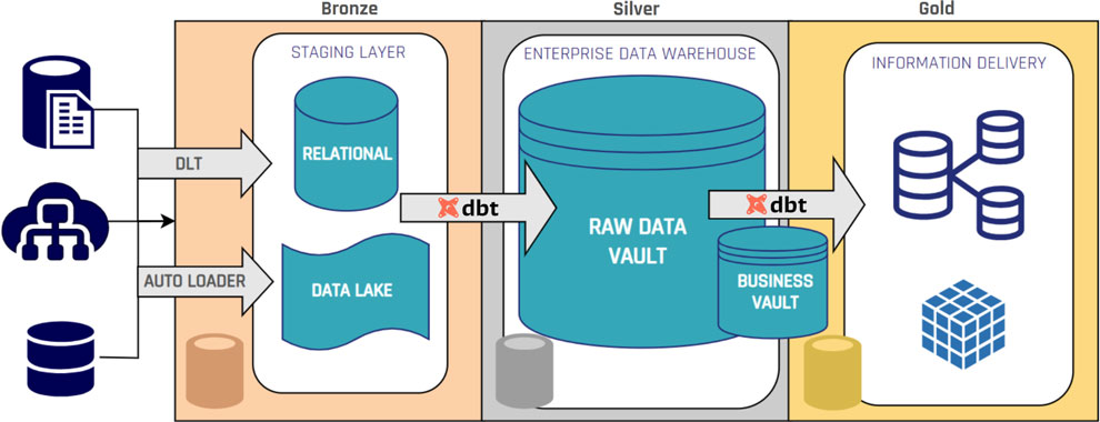
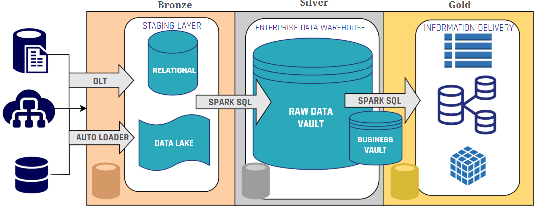
Integrating Data Vault with the Medallion Architecture allows for a synergistic approach, as we can see in image 3.

Data Vault and Medallion Architecture

Image 3: Data Vault and Medallion Architecture

The Bronze layer serves the same purpose as Data Vault’s Staging Area, where raw data is ingested from the different sources and stored in a single place. From then on, the Silver layer will store the Raw Data Vault, source tables will be split into hubs, links, and satellites. Here we can already consider some Databricks’ features, such as schema enforcement for integrity; and also Delta Live Tables and Spark SQL to maintain steady loading processes and automate quality checks. The Business Vault, which derives additional business-relevant data structures, sits between Silver and Gold layers, assisting with the information delivery process.

In the Business Vault, Databricks features such as Z-Ordering and data skipping can optimize performance by organizing data more efficiently. Additionally, Spark SQL can be used for aggregations and transformations supported in PIT and Bridge tables. Finally, in the Gold layer, we can start creating our Information Marts with Flat & Wide structures that improve the performance when querying the information out of the Vault.

Privacy and Security

Databricks’ data governance features included in Unity Catalog can optimize Data Vault implementations by simplifying security and privacy controls. Unity Catalog’s fine-grained access control and data masking capabilities can eliminate the need for satellite splits traditionally used to manage sensitive data. Additionally, the lakehouse architecture enables direct data querying, which facilitates compliance with GDPR and data privacy regulations, particularly for responding to data subject access requests (DSAR) and right-to-be-forgotten requests. These data governance features help to simplify the Data Vault model and reduce the final amount of tables in the Vault.

Historization

While both Data Vault and Databricks offer mechanisms for data historization, relying solely on Delta Lake’s Time Travel for historization in a Data Vault implementation on Databricks might not be the best choice. In Databricks, the VACUUM command can permanently delete older data files, potentially removing historical data needed for auditing, lineage analysis and regulatory compliance. Hence, alternative historization methods should be considered, such as maintaining traditional historization with Data Vault’s modelling insert-only approach, or leveraging Databricks’ Change Data Feed to capture a stream of changes made to Delta Lake tables. This ensures a complete and auditable history, even if older data versions are removed by the VACUUM command.

Performance Considerations

When implementing Data Vault on Databricks, performance optimization requires architectural considerations that comprehend the characteristics of both systems. The modular design of Data Vault can create numerous tables with complex join patterns, which can be challenging in Databricks’ Spark environment, since Delta Lake’s column-based Parquet files can struggle with extensive joins. To address this challenge, practitioners should minimize satellite splits (leveraging Databricks’ native security and privacy features instead), implement virtualization in the Business Vault through views, and utilize Point-in-Time and Bridge tables to precompute historical snapshots that reduce join complexity and aid in achieving the target granularity.

For optimal performance, information marts should adopt Flat & Wide structures that prioritize query speed over storage efficiency (an acceptable trade-off given today’s relatively low storage costs). Additional performance gains can be achieved by strategically applying Delta Lake features like Z-Ordering and data skipping to enhance the information delivery process. The decision between views and fully materialized information marts is also an aspect to consider; while views reduce redundancy and simplify management, materialized marts with denormalized tables provide substantial performance benefits for complex reporting scenarios that would otherwise require resource-intensive joins across multiple Data Vault structures. A balanced approach combining views and materialized views should be based on query complexity, data volume, and update frequency, ensuring that reporting, and analytics workloads remain performant. This way we ensure that a Data Vault implementation on Databricks can maintain both the modeling flexibility of Data Vault and the performance capabilities of the Databricks platform.

Data Vault on Databricks: The Best of both Worlds

Implementing Data Vault on Databricks represents a practical and effective combination that merges Data Vault’s tool-agnostic architecture with Databricks’ technical capabilities. To optimize this integration, organizations should make thoughtful adjustments that create synergies between the modeling methodology and platform, including leveraging Unity Catalog for security and privacy satellite management, combining architectural designs while maintaining historization and data lineage, and virtualizing queries in the downstream layers with Flat & Wide structures with PIT and Bridge tables as underlying elements to enhance performance. This balanced approach allows organizations to improve governance and simplify data management, while preserving the core strengths of both systems.

Column Propagation in Coalesce: Handling IT Table Changes

How Coalesce Manages Column Propagation

Change is inevitable in data management. Whether you like it or not, IT table structures evolve due to various reasons. When these changes occur, they can impact data pipelines, potentially leading to inefficiencies or even failures. Fortunately, coalesce.io offers a robust solution to manage column propagation seamlessly.


Why Do Table Structures Change?

Changes in database table structures can occur for several reasons:

  • Change in the source system: New data sources, modifications in existing systems, or upgrades can introduce changes.
  • Change in the data ingestion process: Adjustments in ETL (Extract, Transform, Load) or ELT (Extract, Load, Transform) processes may require modifications in tables.
  • Development mistakes: Incorrect data modeling, schema design flaws, or unintended changes can also trigger table updates.

Types of Table Structure Changes

Table modifications generally fall into three categories:

  • New Attributes: Additional columns were introduced to capture new data.
  • Removed Attributes: Deprecated or unnecessary columns are being eliminated.
  • Changed Datatypes: Modifications in column data types for compatibility or optimization.

Impact of Changes in IT Tables

The consequences of these changes can vary widely:

  • Best Case: Unused and unabsorbed data, leading to inefficiencies but not immediate failure.
  • Worst Case: Complete pipeline failure, causing data loss or system downtime.

Column Propagation in Coalesce

Coalesce simplifies the process of managing table changes through an efficient column propagation mechanism.

How Column Propagation Works

Column propagation in coalesce.io follows a structured approach:

  1. Select Column: Identify the column that has been added, removed, or modified.
  2. Propagate Addition or Deletion: Ensure that the column change is applied throughout the pipeline.
  3. Mark Downstream Objects: Identify downstream objects that are affected and should be updated accordingly.
  4. Create Commit: Finalize the changes with a commit to reflect them across the system.

Benefits of Using Coalesce for Column Propagation

By leveraging Coalesce’s column propagation features, data engineers can:

  • Automate schema changes: Reduce manual intervention and minimize errors.
  • Ensure data consistency: Prevent mismatches between schema and data models.
  • Improve efficiency: Accelerate change implementation without disrupting workflows.
  • Enhance visibility: Gain better control over how changes impact the entire data pipeline.

Final Thoughts

Managing table changes is a critical aspect of data engineering. With coalesce.io, data teams can seamlessly handle column propagation, ensuring minimal disruptions and optimal performance. Whether you’re dealing with new attributes, removed attributes, or datatype modifications, coalesce.io streamlines the process and enhances data reliability.

Watch the Video

Data Streaming in Snowflake

Data Streaming in Snowflake

In this newsletter, we’ll provide an overview of the possibilities for streaming data using Snowflake.

The approaches discussed here focus on how Snowflake’s features and capabilities enable ingestion and processing data streams with a certain speed. The goal is to explore how businesses can create an advantage by using real time data to make time critical decisions, improve operational efficiency, and enhance customer experiences. Additionally, we’ll examine Snowflake’s architecture to enable a reliable solutions base, its suitability for streaming workloads, and the challenges it addresses.

Data Streaming in Snowflake

This webinar on February 11th, 2025, 11 am CET, shows you how to speed up data-driven decisions using Snowflake’s real-time data capabilities. Learn to unify batch and streaming data pipelines to handle large volumes of data with Snowpipe Streaming, Hybrid Tables, and Dynamic Tables. Discover how to get low-latency insights and make faster decisions without affecting your existing processes. We’ll explore real-world examples of how others use real-time data for dashboards, customer experiences, and more, plus best practices for ensuring data quality and performance. Ideal for data engineers and architects, this session will show you how Snowflake can revolutionize your analytics and help you thrive in today’s fast-paced digital world.

Watch Webinar Recording

What to Expect

You will gain an overview of the various built-in tools and techniques Snowflake provides to handle real time data streaming, including data ingestion, processing, and querying capabilities. We’ll cover Snowflake’s architectural components, such as tables, views, and processing capabilities, and explore how they are used to managing transactional workloads.

The main focus of this blog is to provide insights on how Snowflake enables real time data processing, the opportunities it presents, and the trade-offs to consider when implementing streaming solutions.

Real Time Data – an Overview

Real time data enables businesses to process information immediately after it is generated. Unlike traditional batch processing, which works with fixed intervals, real time data flows continuously, allowing for dynamic and immediate actions. This type of data processing has become increasingly important for organizations seeking to stay competitive in a fast-moving market.

Key Characteristics of Real Time Data

Real time data has distinct characteristics that differentiate it from other types of data flows:

  • High Velocity: Data is processed at high speeds, often within milliseconds or seconds.
  • Low Latency: Systems are designed to minimize delays, ensuring timely access to insights.
  • Dynamic Streams: Continuous and often unpredictable data streams require flexible and scalable processing.

Each of these characteristics brings unique advantages and challenges to the table. For this reason, organizations need specialized tools and platforms to handle real time data effectively.

Why Real Time Data is Important

The value of real time data lies in its ability to provide immediate insights, which enable organizations to act without delay. It can significantly enhance several business areas, such as:

  • Enhanced Decision-Making: Real time insights enable proactive responses, such as dynamically adjusting pricing or inventory based on live demand.
  • Customer Personalization: By analyzing behavior in real time, companies can deliver tailored experiences that meet customer expectations in the moment.
  • Operational Efficiency: Constant monitoring helps organizations to detect and address issues early, reducing downtime and optimizing performance.
  • Risk and Fraud Detection: Rapid identification of anomalies or threats reduces exposure to fraud and operational risks.

The benefits of real time data are clear; however, its implementation comes with specific challenges, as detailed below.

Challenges with Real Time Data

While the advantages of real time data are significant, they are accompanied by a unique set of challenges:

  • Handling Velocity and Volume: Processing large streams of data at high speed requires scalable systems.
  • Ensuring Consistency: Maintaining data accuracy across distributed systems can be complex, especially when dealing with multiple sources.
  • Integration Complexity: Real time data must often be combined with batch systems or legacy analytics, which introduces technical complexities.

The continuous flow and immediacy of real time data make it indispensable for businesses aiming to stay ahead in their industries. With the right tools and architecture, organizations can unlock its potential to deliver significant value and competitive advantage.

Real Time Data in Snowflake

Snowflake offers a modern approach to handling real time data by combining its cloud-native architecture with features designed for continuous ingestion, processing, and querying. With built-in tools like Snowpipe, streams, and tasks, Snowflake enables organizations to integrate real time data. In this section, we are going to explore how Snowflake manages real time data and its possibilities to meet the demands of streaming workloads.

Snowflake’s Architecture for Real Time Data

Snowflake’s architecture combines shared-disk and shared-nothing concepts. It uses a central, cloud-based data repository (the “shared-disk” portion) while compute resources (virtual warehouses) scale independently and process data in parallel (the “shared-nothing” aspect).

  • Batch: Traditionally, data engineers batch large amounts of data into Snowflake using the COPY command or scheduled loads. The compute layer scales up for heavy loads and then scales back down for cost efficiency.
  • Real Time: Continuous ingestion focuses on small, frequent data arrivals. The architecture still benefits from the separation of storage and compute, allowing Snowflake to handle real time feeds without blocking batch workloads or analytics queries.

Micro-partitions

Snowflake automatically divides tables into micro-partitions, compact storage units that group data based on natural ordering or load patterns.

  • Batch: Micro-partitions shine when running large analytical queries, as Snowflake can prune out unnecessary partitions quickly, boosting performance for wide-ranging queries.
  • Real Time: Frequent data loads generate more micro-partitions. The fine-grained organization remains beneficial, but you need to plan for slightly more overhead in terms of partition management, particularly if your real time data streams produce extremely high volumes.

Dynamic and Hybrid Tables

Speaking of tables, the next two entities are very helpful when considering processing real time data in Snowflake.

Dynamic Tables allow you to define continuous transformations within Snowflake. Think of them as similar to materialized views, but more flexible and with the ability to handle complex transformations and dependencies. You specify a SQL query for how the table should be built, and Snowflake automatically processes incremental changes from source tables behind the scenes.

  • Incremental Data Processing: Instead of running ad-hoc or scheduled jobs, Dynamic Tables automatically update when new data arrives. You can set a target lag by specifying a refresh duration or defining a downstream dependency. Within the downstream dependency, the last dynamic table determines when the data needs to be refreshed.
  • Continuous Pipelines: They reduce the need for manual orchestration with Snowflake Tasks or external job schedulers.
  • Complex Transformations: Unlike materialized views (which are generally suited for simpler aggregates), Dynamic Tables can handle joins, window functions, and other advanced SQL operations.


Hybrid Tables are a newer concept that merges Snowflake’s columnar micro-partition storage with row-oriented features, making it easier to handle fast, high-volume inserts or updates. They aim to support both analytic (OLAP) and transactional (OLTP-like) workloads in a single Snowflake environment.

  • Faster Row-Level Operations: Traditional Snowflake tables can handle inserts and updates at scale, but they’re optimized primarily for analytical reads. Hybrid Tables aim to make row-level operations more efficient.
  • Mixed Workload Support: Combine real time event ingestion (often associated with row-level databases) and analytical querying (where column-based storage excels).
  • Reduced Latency: By better handling small transactions and frequent data changes, Hybrid Tables can help lower the time it takes to get new data ready for querying.

Snowpipe and Snowpipe Streaming

Snowpipe is Snowflake’s continuous data ingestion service that loads data from external or internal stages. Typically, you point Snowpipe at a cloud storage location (e.g., Amazon S3) where new files land, and it automatically imports them.

  • Classic Batch: The COPY command is often scheduled to run at fixed intervals (e.g., hourly or daily), which can introduce latency.
  • Snowpipe: Instead of waiting for a scheduled batch, Snowpipe automatically pulls in smaller file increments soon after they arrive in the stage. This reduces the time between data generation and availability for queries.

However, Snowpipe is optimized for continuous loads of small files – think micro-batches, rather than large single-file loads. If your data volume spikes significantly, you might face higher costs or need to switch to different ingestion strategies to maintain throughput.

Snowpipe Streaming is an API-based approach that writes data directly to Snowflake tables, bypassing intermediate storage altogether. This can reduce latency and loading times even further than standard Snowpipe.

Why is it “More Real Time”? Data arrives instantly (or very close to it) in Snowflake, enabling near real time reporting. You don’t need to wait for batch files to land in cloud storage, and it’s often more cost-effective at scale, especially for high-frequency, small data events.

Additionally, the Snowflake Connector for Apache Kafka supports Snowpipe Streaming, allowing a near-seamless way to flow messages from Kafka topics straight into Snowflake tables. This integration is a significant step toward bridging the gap between streaming data platforms and Snowflake’s cloud data warehouse.

Snowflake Streams

Lastly, a Snowflake “Stream” tracks changes made to a table (inserts, updates, and deletes). This is particularly useful for Change Data Capture (CDC) workflows, enabling efficient processing of real time data.
You can design pipelines that react to these CDC streams, triggering transformations or downstream processes. This is ideal for scenarios where real time data updates must flow into transactional or operational systems.

Limitations and Possibilities of Real-Time Data in Snowflake

After breaking down some key factors, we will examine several limitations and possibilities when working with Snowflake and real time data.

While Snowflake aims for near real time processing, it isn’t designed as an ultra-low-latency, sub-second event-processing engine. Rapid, continuous ingestion can drive up costs if you’re not careful with warehouse sizing and auto-suspend settings. Each warehouse or streaming component could incur charges for frequent queries and data loads.

Monitoring multiple data streams, scaling them and managing their throughput can be complex. You’ll need robust DevOps and DataOps practices to ensure data integrity and consistent performance.

On the other hand, you can enable real time dashboards and analytics. With Snowpipe Streaming and the Kafka Connector, you can feed data directly into Snowflake and power dashboards that update within seconds or minutes. CDC streams enable event-driven pipelines where changes in your transactional databases trigger immediate actions in Snowflake, such as downstream transformations or alerts. Snowflake’s separation of storage and compute makes it easier to handle spiky workloads. Real time pipelines can scale up independently of other batch or analytical tasks, ensuring smooth parallel processing.

Many organizations mix real time flows with traditional batch loads. Snowflake’s architecture can accommodate both simultaneously without conflict.

Conclusion

By bringing together Hybrid Tables for row-based writes, Snowpipe Streaming for near real time ingestion, Snowflake Streams for continuous change detection, and Dynamic Tables for automated transformations, organizations can introduce real time data flows on top of their existing batch approach. This collaboration of Snowflake features opens up opportunities to capture high-velocity data and process it almost immediately, enabling decision-makers to access live metrics, personalize customer interactions as they happen, optimize operational processes, and detect anomalies or fraud with minimal delay. When combined with standard batch ingestion, this architecture preserves historical data and large-scale analytics while adding a complementary layer for low-latency, event-driven insights.

However, there are challenges and limitations to consider. More frequent writes can drive up compute costs, especially if data arrives at unpredictable volumes and velocities. Ensuring consistent data models becomes trickier if schema changes occur rapidly, as real time pipelines need to keep up with adjustments in source systems. Hybrid Tables, while excellent for rapid inserts, may not always yield the same query performance as columnar tables when it comes to large-scale analytical workloads; likewise, the cost overhead of always-on streaming pipelines can be significant if not carefully sized and monitored. Complexity also rises with more moving parts, and a robust DataOps or DevOps framework is critical for controlling ingestion, transformation, and monitoring across multiple modes of data processing.

Still, integrating these real time capabilities into an existing batch-loading architecture can be done gradually by setting up a dedicated real time pipeline that feeds into Snowflake alongside the traditional bulk loads. The new pipeline could ingest event data using Snowpipe Streaming and store it initially in Hybrid Tables, where Streams and Dynamic Tables can process changes in near real time. Historical data loads and heavy analytical queries would continue using the existing batch approach with columnar, micro-partitioned tables. Over time, teams can merge both approaches at the consumption layer—whether in BI dashboards, ML pipelines, or operational analytics—to combine the immediacy of real time data with the depth of historical context, all within the same Snowflake ecosystem.

Microsoft Fabric as an Enterprise Data Platform

Intelligent Data Front-ends

Introduction to Microsoft Fabric and dbt Cloud

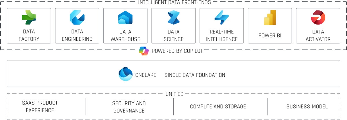
In today’s digital world, organizations need a unified, scalable, and collaborative data platform to power analytics, AI-driven insights, and business intelligence. Enter Microsoft Fabric—a comprehensive, role-based, SaaS-delivered data platform that brings together key Azure services under a single “one lake” foundation with built-in AI capabilities.

In this article, we’ll explore how Microsoft Fabric can serve as your enterprise data platform, how it integrates with data modeling tools like dbt Cloud, and a proven “medallion” reference architecture that takes you from raw data ingestion to business-ready information marts. We’ll also discuss future extensions, practical limitations, and best practices to guide your journey.

Microsoft Fabric as an Enterprise Data Platform

This webinar covers leveraging Microsoft Fabric to implement a modern, end-to-end data platform. You will learn, how the different Fabric services can be combined, to implement a medaillon architecture, supported by Data Vault 2.0 and dbt Cloud. A live demo will show lakehouses, warehouses, and Hub, Links, and Satellites in a real world scenario!

Watch webinar recording

Quick Primer: The Data Vault Methodology

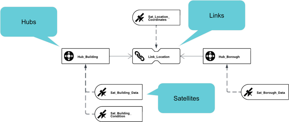
Before diving into Fabric, it’s helpful to understand the Data Vault approach—an architecture pattern that brings agility, auditability, and scalability to your data warehouse. It comprises three core components:

  • Business Keys: Unique identifiers of business objects (e.g., customer number in a CRM).
  • Descriptive Data: Attributes that describe business keys (e.g., customer name, birthdate), which evolve over time.
  • Relationships: Linkages between business keys (e.g., customer–order relationships in a CRM).

By separating these elements into hubs, satellites, and links, Data Vault provides a repeatable, auditable framework for loading and tracing data lineage, perfectly suited for modern cloud platforms.

hubs, links, and satellites

Microsoft Fabric: Core Front-Ends and Services

At its heart, Microsoft Fabric brings together seven role-based “front-end” experiences, but three of them are key to enterprise data engineering and warehousing:

Data Factory

  • Data Flows: Low-code transformations (joins, aggregations, cleansing) via a Power Query-like interface.
  • Data Pipelines: Petabyte-scale ETL/ELT workflows with full control-flow constructs (if/else, loops).

Use case: Ingest raw data from relational, semi-structured, or unstructured sources into your landing zone lakehouse.

Data Engineering

  • Lakehouses: Unified storage for structured/unstructured data in Delta-Parquet format, with SQL endpoints for analytics.
  • Notebooks: Interactive Python, R, or Scala environments for data prep, analysis, and data science exploration.
  • Spark Job Definitions: Batch and streaming ETL jobs on Spark clusters.
  • Data Pipelines: Orchestrated sequences of collection, processing, and transformation steps.

Use case: Land raw data and expose it to data scientists or further transformation processes.

Data Warehouse

  • Warehouses: Relational-style databases with Delta-Parquet storage, instant elastic scale, and full transactional support.
  • Support for cross-warehouse queries and seamless read access to lakehouses.

Use case: Implement Data Vault’s Raw Vault, Business Vault, and Information Marts for BI consumption.

Intelligent Data Front-ends

Workspaces

All Fabric resources live inside workspaces, which group lakehouses, warehouses, notebooks, pipelines, and more. Workspaces enable:z

  • Role-based access control and collaboration
  • Integration with Git for versioning and CI/CD
  • Cross-workspace data access via shortcuts

Integrating dbt Cloud with Microsoft Fabric

dbt Cloud is an industry-leading transformation framework that brings software engineering best practices to your data models: modular SQL, testing, documentation, and CI/CD. In Fabric, dbt Cloud:

  • Connects to a Fabric workspace as a data warehouse endpoint
  • Generates SQL models (SELECT statements), reading from lakehouses or warehouses
  • Executes those models natively on Fabric warehouses

Key benefit: dbt manages your Data Vault layers (hubs, links, satellites, and information marts) with clear lineage, testing, and version control—while Fabric handles execution, storage, and compute elasticity.

Reference Architecture: The Medallion Approach on Fabric

The modern “medallion” architecture separates data into three refinement layers—Bronze (raw), Silver (conformed/business), and Gold (BI-ready). Here’s how it maps onto Fabric:

Bronze (Landing Zone Lakehouse)

Data Factory pipelines copy raw relational, JSON, and unstructured files into a lakehouse. This fully persisted, immutable history remains read-only for most users.

Silver (Raw &amp; Business Vault Warehouses)

  • Raw Vault Warehouse: dbt models generate staging views/tables with hash keys, load dates, and audit metadata.
  • Business Vault Warehouse: dbt builds hubs, links, and satellites based on business keys and relationships.

Gold (Information Mart Warehouse)

Information marts—star or snowflake schemas—are created via dbt models as optimized, query-ready tables for BI tools (Power BI, Tableau, etc.).

Dbt Cloud and Microsoft Fabric - Medaillon

Live Demo Highlights

During our webinar demonstration, we walked through:

  • Setting up a Fabric workspace and viewing lakehouse tables via SQL and the Windows Explorer integration
  • Using a Data Factory pipeline to ingest sample Snowflake data into a landing zone lakehouse
  • Authoring dbt models in dbt Cloud to create staging (hashing, load dates), hub tables, link tables, and satellites
  • Executing dbt runs that generate and run SQL in Fabric warehouses, and previewing results directly in the Fabric UI
  • Accessing all data files and Delta-Parquet tables seamlessly in Windows Explorer for multi-cloud portability

Outlook: Next-Gen Enhancements

Beyond the core implementation, here are exciting ways to evolve your Fabric-dbt platform:

  • Workspace Segmentation & Data Mesh: Create dedicated workspaces for medallion layers or business domains, and stitch multiple dbt projects together with dbt Mesh for a true data mesh design.
  • Real-Time Data Integration: Leverage Fabric’s built-in streaming capabilities to blend real-time feeds into your warehouses alongside batch data.
  • Enhanced Governance & Semantic Layers: Define and enforce semantic models both in dbt and in Fabric (via semantic models) to ensure consistent metrics across all BI tools.
  • Data Science Collaboration: Grant read-only access to bronze lakehouses and empower data scientists to use Fabric notebooks (Python, R, Scala) for ad-hoc analysis and advanced ML experiments.
  • Simplified Migration: Existing dbt projects on on-prem or other cloud warehouses can be repointed to Fabric with minimal code changes—especially when using community macros for Data Vault deployments.

Considerations & Limitations

While Fabric is powerful, be mindful of:

  • Write Support: Lakehouses currently support only SQL writes—transformations must target Fabric warehouses.
  • Shortcut Management: Cross-workspace shortcuts must be manually maintained; frequent schema changes can add overhead.
  • Multiple Overlapping Tools: Data Factory, Data Engineering pipelines, notebooks, and dbt all offer ETL—establish clear standards to avoid confusion.
  • Product Maturity: As a relatively new platform, UI changes and minor bugs may appear; plan for iterative improvements.
  • Capacity Transparency: Compute and storage share capacity; monitor and size your Fabric capacity carefully to meet SLAs.

Conclusion

Microsoft Fabric, coupled with dbt Cloud, delivers an end-to-end Enterprise Data Platform that unifies data ingestion, storage, transformation, and consumption. By applying proven patterns like the medallion architecture and Data Vault methodology, you can build a scalable, collaborative, and governed environment, empowering both data engineers and business users to unlock insights faster.

Ready to take your data platform to the next level? Reach out for a tailored workshop, architecture advisory, or hands-on implementation support.

Creating Data Vault Stages

Data Vault Stages

The Data Vault methodology provides a robust framework for managing and organizing enterprise data. One of the foundational components of a Data Vault is the stage. In this guide, we’ll explore what Data Vault stages are, their importance, and how to create them effectively.


Understanding Node Types in Data Vault

Before diving into stages, let’s review the key node types in a Data Vault:

  • Stages: Temporary storage areas where raw data is preprocessed.
  • Hubs: Central entities containing unique business keys.
  • Links: Relationships between hubs.
  • Satellites: Contextual and descriptive data for hubs and links.
  • PITs (Point-in-Time Tables): Optimized query performance tools.
  • Snapshot Tables: Historical states of data.
  • Non-Historized Links & Satellites: Used when historical tracking isn’t required.
  • Multi-Active Satellites: Support multiple active records for the same key.
  • Record Tracking Satellites: Track changes and versions of records.

Features of Data Vault Patterns

The Data Vault methodology leverages years of practical experience to deliver several key features:

  • Patterns Based on Expertise: Proven methods for efficient loading and processing.
  • Multi-Batch Processing: Handle multiple data batches simultaneously.
  • Automatic PIT Cleanup: Uses logarithmic snapshot logic for optimal performance.
  • Virtual Load End-Date: Allows insert-only processes by using calculated end dates.
  • Automated Ghost Records: Simplifies handling of missing or incomplete data.

Why Are Stages Important in Data Vault?

Stages play a critical role in the Data Vault architecture by enabling efficient data preparation and ensuring data integrity. Key benefits include:

  • Hash Keys & Hash Diffs: Ensures unique identifiers for data integration and deduplication.
  • Load Date & Record Source: Tracks the origin and timing of data entries.
  • Prejoins: Combines data efficiently before entering the vault.
  • Hard Rules: Implements strict validation and transformation logic.

How to Create a Data Vault Stage

Creating a stage in a Data Vault involves leveraging the right tools and techniques. For this, we recommend using Datavault4Coalesce, a powerful platform designed for Data Vault implementation. This tool simplifies the process by automating key tasks and ensuring best practices are followed.

Conclusion

Stages are a foundational component of the Data Vault methodology, enabling seamless data preparation and integration. By understanding their role and leveraging the right tools, you can ensure the success of your Data Vault implementation.

Watch the Video

Custom Node Types in Coalesce

Custom Node Types in Coalesce: Unlocking Flexibility and Reusability

Nodes are the foundational building blocks in coalesce.io, serving as database objects like tables or views. Each node belongs to a specific type, equipped with a predefined user interface, a create template, and a run template. While coalesce.io provides four standard node types, custom node types allow users to adapt and extend these capabilities for unique requirements.


What Are Custom Node Types?

Custom node types enable users to define reusable database object patterns. By specifying a user interface (UI), Data Definition Language (DDL), and Data Manipulation Language (DML), users can create tailored solutions for patterns such as stages, dimensions, facts, hubs, and links. Parameters and macros make these custom types even more adaptable and reusable.

Why Create Custom Node Types?

Custom node types address two key needs:

  • Custom Needs: Standard node types may not cover specific use cases.
  • Reusability: Custom node types eliminate the redundancy of repeatedly creating similar nodes, saving time and effort.

Key Components of Custom Nodes

Node Definition and UI Configuration

The node definition specifies the UI elements, such as materialization selectors, toggles, dropdowns, and text boxes. These components define how users interact with and configure the custom node.

Create Template

The create template includes SQL logic for generating tables or views. It supports column transformations, comments, clustering keys, and all Snowflake DDL features.

Run Template

The run template defines DML operations, such as inserting data, applying incremental or merge strategies, and performing transformations. These operations are executed exclusively for table-based nodes and utilize all Snowflake DML features.

Get Started with Custom Node Types

Custom node types in coalesce.io empower teams to design reusable, scalable solutions tailored to specific needs. By leveraging their flexibility, you can streamline development, reduce repetitive tasks, and maximize efficiency in your data workflows.

Watch the Video

Close Menu