search
0
All Posts By

Jan Paul Langner

Jan Paul Langner is a Senior Business Intelligence Consultant at Scalefree specializing in Data Vault 2.0 and cloud native automation. A CDVP2 and SnowPro Core professional, he recently led the development of a near real-time (NRT) data platform for international leading companies in the industrial technology sector using Snowflake and dbt. Jan Paul combines technical expertise in Python and Kafka with a Scrum Master mindset to deliver high performance, scalable data architectures.

Monitoring of a Snowflake Powered EDW

Snowflake Built-In Tools

Introduction to Snowflake

Snowflake established itself as one of the most widely used cloud data platforms, providing a scalable and flexible architecture for building, maintaining, and operating Enterprise Data Warehouses. While it aims to eliminate data silos and simplify the data structure, with billions of queries a day (overall), its elastic computing handles the workload for good performance and a satisfied customer.

However, as organizations rely increasingly on Snowflake, monitoring their solution might be crucial for performance optimization, error and root cause analysis, and cost control. Although Snowflake handles these tasks very well on its own, experience shows some need for human interference when it comes to more complex queries, to increase performance, lowering the runtime without upscaling or scaling out.

This blog article aims to provide general information about and technical insights into Snowflake. Focusing on techniques as well as built-in tools to analyze bottlenecks, we aim to potentially increase performance and therefore decrease unnecessary costs.


Snowflake Built-In Tools

Query History

Starting with Snowflake’s built-in tools, we will dive into its roots and combinations of several metrics.

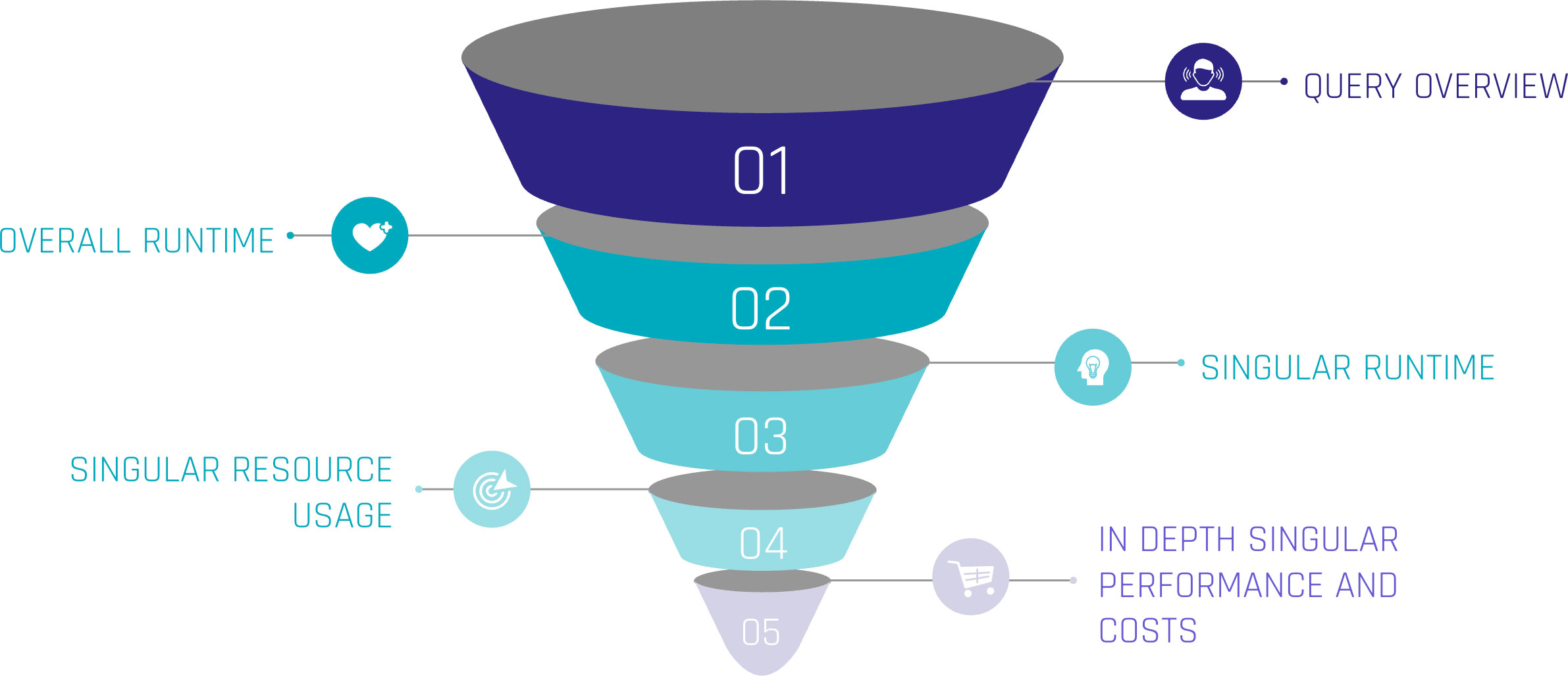
Monitoring query performance includes several depths of insight, from an overview of the general query history, down to the performance of each individual step within a query.

Snowflake Built-In Tools

Let’s assume the top level as an overview of our queries. Including metrics such as:

  • Start Time,
  • Total Time,
  • Status and
  • Query Type.

For the first level, we can gain insights when the queries start, how much time they were consuming, whether they succeeded or failed, or even are still running. Lastly, we can see the type of query, such as ‘CREATE TABLE’, ‘INSERT’, or ‘SELECT’. At this level, a brief overview could be created about the traffic within the Warehouse.

When hearing about this, you may be familiar with a built-in tool called ‘Query History’, which tracks this kind of information automatically without the need for user interference. It is easily available within the sections ‘Monitoring’ and ‘Query History’.

Query Profile

Further, it is easily possible to extract more information about the executed queries. Every single query within the ‘Query History’ has a unique identifier and attached metrics. Within the ‘Query History’ section, when choosing a query by simply clicking on it, we gain insights into the single query. These include two main sections.

‘Query Details’ delivers information about the query in general. Including the above-mentioned ‘Start Time’, ‘End Time’, ‘Warehouse Size’, and ‘Duration’, which is divided into ‘Compilation’, ‘Execution’, and further time-consuming steps.

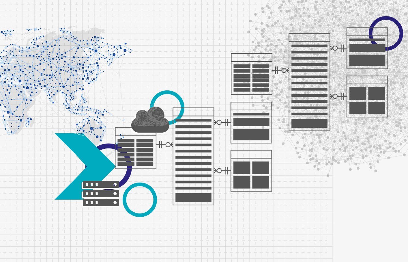
‘Query Profile’ describes the execution plan of the query as a graphical representation. Each step within the query, such as ‘SELECT’, ‘JOIN’, and ‘WHERE CONDITION’ are represented as nodes within the graph. These nodes are operations, triggered by the query. Each fulfilling a task like filtering data, selecting data rows, but also scanning results, and reading data from cache. Snowflake interprets the written SQL and creates a performant execution plan by itself.

Despite that, each node consumes more or less resources, depending on the SQL code itself, the underlying dataset, and the Warehouse configurations. Using the ‘Query Profile’, we can identify the most time-consuming steps in our query, such as false ‘JOINS’, and work around those nodes to identify more performant solutions. Therefore, the ‘Query Profile’ provides detailed information about each node, like processing time, cache scanning, and partition pruning. For further information, check out the Snowflake Documentation.

Custom Monitoring Solution

But when Snowflake already provides a solution, why do we need separate monitoring?

Although already delivered, your requirements may vary from the existing solution. With the built-in tools mentioned above, the possibility to check on each query is given. Additionally, Snowflake may not be the only tool used for data processing. ELT tools like dbt or Coalesce help data engineers improve processes. To include these further metrics from outside Snowflake, a custom monitoring solution, based on Snowflake’s delivered metrics, is needed.

With this in mind, the following section focuses on our own scalable monitoring solution.

Account Usage and Information Schema

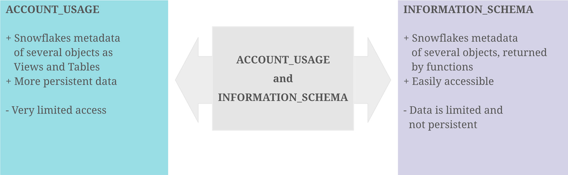
With the idea that the data of the graphical output exists as a table or view, containing all data necessary, it turns out that Snowflake provides us the schemas ‘ACCOUNT_USAGE’ and ‘INFORMATION_SCHEMA’, fulfilling this purpose. They provide similar opportunities for this challenge, although there are some differences.

‘ACCOUNT_USAGE’ provides insights into Snowflake metadata of several objects. This includes ‘QUERY_HISTORY’, which contains the information described in the sections above. The query history is available for all queries within the last 365 days. This enables the loading of metrics entities in the Data Warehouse, making the information readily accessible and persistent for daily, weekly, or monthly processes. The downside is that access to the ‘ACCOUNT_USAGE’ schema is often limited.

The ‘INFORMATION_SCHEMA’ contains a set of system-defined views and tables, providing metadata and information about created objects. Using predefined functions on the ‘INFORMATION_SCHEMA’, metadata can be retrieved, which, on the other hand, is limited to some factors. As this option is more accessible for developers, the focus remains on this option.

Account Usage and Information Schema

Extract Metrics Data

At the beginning, it is crucial to point out the limitations and possibilities of this approach. For the scope of this blog, two functions on the ‘INFORMATION_SCHEMA’ are needed.

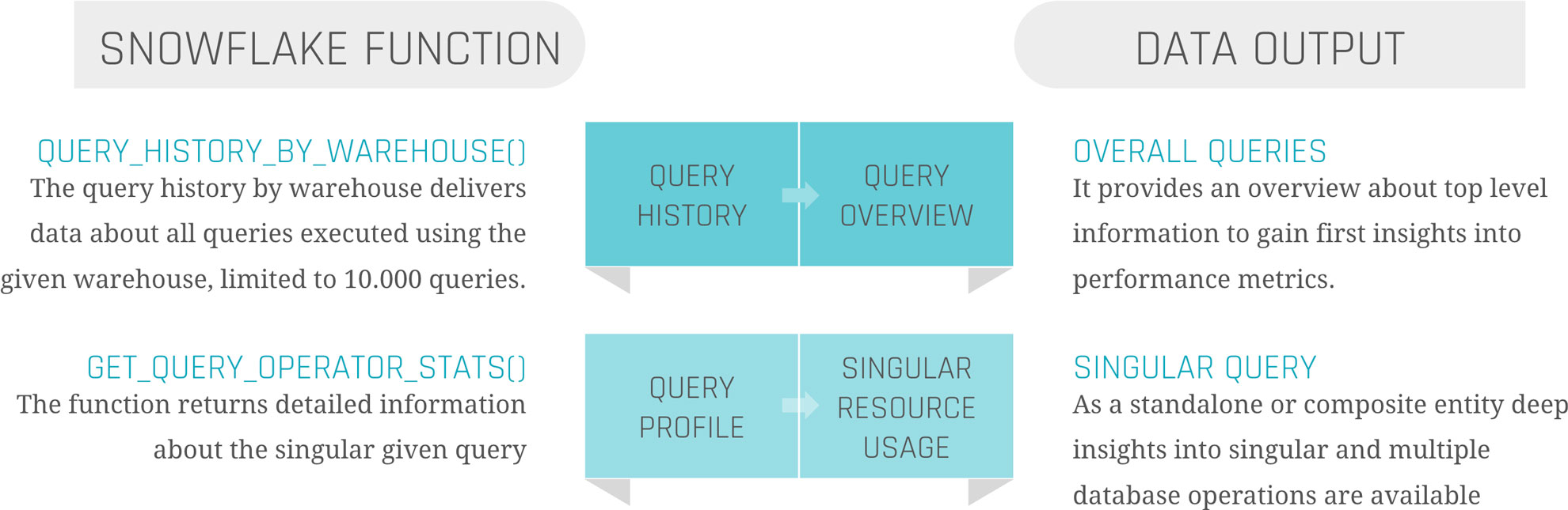
‘QUERY_HISTORY_BY_WAREHOUSE()’ is equal to ‘QUERY_HISTORY’.

‘GET_QUERY_OPERATOR_STATS()’ is the equivalent of ‘QUERY_PROFILE’.

‘QUERY_HISTORY_BY_WAREHOUSE()’ takes four different arguments.

  • ‘WAREHOUSE_NAME’ – The name of the Warehouse executing the queries
  • ‘END_TIME_RANGE_START’ – Time range within the last 7 days, in which the query started running
  • ‘END_TIME_RANGE_END’ – Time range within the last 7 days, in which the query completed running
  • ‘RESULT_LIMIT’ – The number of the maximum returned rows. The default lies by ‘100’, the range by ‘1’ to ‘10.000’

The output is the ‘QUERY_HISTORY’ as a structured table with some extra information. Each query is displayed in one row. Therefore, the metrics are aggregated into one specific query.

The most critical limitation seen here is the ‘RESULT_LIMIT’ and ‘END_TIME_RANGE_*’, as it forces us to retrieve the data before the 7-day retention ends and before 10.000 other queries have been executed. Depending on the size of the Warehouse and the scope of the monitoring range, the extract and load process must be customized.

‘GET_QUERY_OPERATOR_STATS()’ takes one argument.

  • ‘QUERY_ID’ – The unique ID of the executed query.

The output is a structured table of the ‘QUERY_PROFILE’ of one specific query. Each step in the execution plan is displayed as one row, so the output size depends on the complexity of the query itself. Each node is detailed with available metadata, breaking down information from ‘GET_QUERY_OPERATOR_STATS()’ into individual steps. This allows for a deeper analysis of performance metrics, helping to identify any bottlenecks.

As the function is on query-level, it is not done by joining the table outputs of those two functions together to get a satisfactory result. Further steps are needed.

Load Metrics Data

Load Metrics Data

Before filtering, transforming, or joining the data, it is suggested to load the data as it comes into persistent tables.

Snowflake Query History

The first step should be to create the table when calling the function, already combining these two components to avoid missing capture data, columns, or false data types. To keep continuous loading, use your preferred ELT tool to append the process at the end, or set up a scheduled Snowflake Task, considering the limitations mentioned above.

Snowflake Query Profile

This process is more complex. To load the data, it is not sufficient to simply call the function once for the query history. To ensure data integrity and a clear 1:n solution (1 row in the query history, n>0 rows in the query profile), it is needed to iterate through the list of all query IDs inside the query history and run the function for each one of them. Each of the resulting datasets needs to be inserted into the corresponding table.

Information Delivery

Now, as the data is extracted and loaded, the last remaining steps are transforming the data and information delivery. As this strongly depends on the use case, we focus on linking the two metrics tables and creating a standard dashboard inside Snowflake to show the results.

Our two tables ‘snowflake_query_history’ and ‘snowflake_query_profile’ are in a soft relation, where the “QUERY_ID” serves as a unique identifier to link each query from the query history to its query profile. Therefore, joining both tables on the “QUERY_ID” is indispensable. The first decision to be made is whether to keep one row for each query and aggregate the object constructs or to split it up into its individual steps, like within the query profile. For simplicity, we focus on the second option to avoid complex SQL statements for the dashboard. As the SQL statement only includes the ‘SELECT’ and ‘JOIN’ operators, you may choose a view as materialization, instead of a table.

With the possibility of creating dashboards out of Snowflake worksheets, it is relatively easy to integrate simple SQL statements into the dashboard, represented as charts. For some examples, we will take a look at the resulting data.

Query Performance

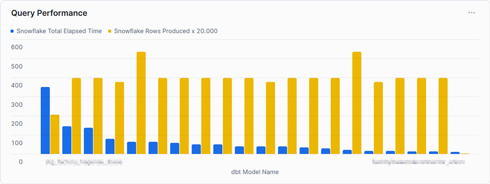
This example shows the top 20 queries by ‘TOTAL_ELAPSED_TIME’, the overall time the query needs to compile, run, waiting time, and other technical steps. As noticed by the chosen x-axis label, Snowflake’s metrics can be combined using other tools, such as dbt. It is set to compare this time against the produced rows to gain some insights into whether the queries can handle much data or not. As can be seen, the query consuming the most time, and therefore credits, does not produce the most rows. At this point, we may be interested in gaining some insights into the query itself.

Query Profile

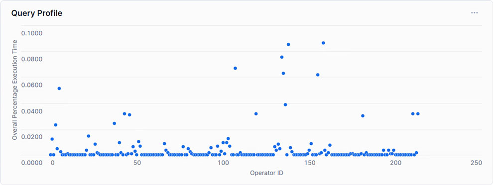
Showing each Operator with its corresponding relative runtime, only a handful exceed 5% of the total execution time. This may indicate that within the SQL statement, only a few steps need to be optimized to create an overall more performant query.

Query Dashboard

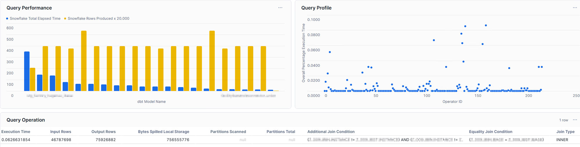
With this in mind, the single query can also be analyzed in the dashboard. For example, you may take into account input rows and output rows, bytes spilled, partitions scanned, and partitions total, or the join condition. Furthermore, you may not only gain insights into your query performance, but also into your table management, such as clustering and partitioning. Additionally, you are also capable of integrating more metrics coming from external sources and linking them directly to Snowflake, making it a powerful monitoring solution.

Conclusion

Snowflake offers a powerful and highly adaptable cloud data platform that meets the demands of modern enterprise data warehousing. However, as data volume and complexity grow, so does the need for proactive monitoring and optimization to ensure continued performance and cost efficiency. By leveraging Snowflake’s built-in tools and implementing strategic performance-enhancing techniques, organizations can address bottlenecks effectively and optimize query performance.

In this article, we addressed the opportunities given through Snowflake’s built-in tools and how to effectively use them. We learned that although these tools are great, to gain a fast and high-level overview, as well as detailed insights at the same time, it is relatively easy to create your own dashboard with the loaded data. Therefore, you are able to analyze and evaluate it, as well as make optimum use of resources to enable high-performance operation without increasing cost by scaling up or scaling out.

Data Streaming in Snowflake

Data Streaming in Snowflake

In this newsletter, we’ll provide an overview of the possibilities for streaming data using Snowflake.

The approaches discussed here focus on how Snowflake’s features and capabilities enable ingestion and processing data streams with a certain speed. The goal is to explore how businesses can create an advantage by using real time data to make time critical decisions, improve operational efficiency, and enhance customer experiences. Additionally, we’ll examine Snowflake’s architecture to enable a reliable solutions base, its suitability for streaming workloads, and the challenges it addresses.

Data Streaming in Snowflake

This webinar on February 11th, 2025, 11 am CET, shows you how to speed up data-driven decisions using Snowflake’s real-time data capabilities. Learn to unify batch and streaming data pipelines to handle large volumes of data with Snowpipe Streaming, Hybrid Tables, and Dynamic Tables. Discover how to get low-latency insights and make faster decisions without affecting your existing processes. We’ll explore real-world examples of how others use real-time data for dashboards, customer experiences, and more, plus best practices for ensuring data quality and performance. Ideal for data engineers and architects, this session will show you how Snowflake can revolutionize your analytics and help you thrive in today’s fast-paced digital world.

Watch Webinar Recording

What to Expect

You will gain an overview of the various built-in tools and techniques Snowflake provides to handle real time data streaming, including data ingestion, processing, and querying capabilities. We’ll cover Snowflake’s architectural components, such as tables, views, and processing capabilities, and explore how they are used to managing transactional workloads.

The main focus of this blog is to provide insights on how Snowflake enables real time data processing, the opportunities it presents, and the trade-offs to consider when implementing streaming solutions.

Real Time Data – an Overview

Real time data enables businesses to process information immediately after it is generated. Unlike traditional batch processing, which works with fixed intervals, real time data flows continuously, allowing for dynamic and immediate actions. This type of data processing has become increasingly important for organizations seeking to stay competitive in a fast-moving market.

Key Characteristics of Real Time Data

Real time data has distinct characteristics that differentiate it from other types of data flows:

  • High Velocity: Data is processed at high speeds, often within milliseconds or seconds.
  • Low Latency: Systems are designed to minimize delays, ensuring timely access to insights.
  • Dynamic Streams: Continuous and often unpredictable data streams require flexible and scalable processing.

Each of these characteristics brings unique advantages and challenges to the table. For this reason, organizations need specialized tools and platforms to handle real time data effectively.

Why Real Time Data is Important

The value of real time data lies in its ability to provide immediate insights, which enable organizations to act without delay. It can significantly enhance several business areas, such as:

  • Enhanced Decision-Making: Real time insights enable proactive responses, such as dynamically adjusting pricing or inventory based on live demand.
  • Customer Personalization: By analyzing behavior in real time, companies can deliver tailored experiences that meet customer expectations in the moment.
  • Operational Efficiency: Constant monitoring helps organizations to detect and address issues early, reducing downtime and optimizing performance.
  • Risk and Fraud Detection: Rapid identification of anomalies or threats reduces exposure to fraud and operational risks.

The benefits of real time data are clear; however, its implementation comes with specific challenges, as detailed below.

Challenges with Real Time Data

While the advantages of real time data are significant, they are accompanied by a unique set of challenges:

  • Handling Velocity and Volume: Processing large streams of data at high speed requires scalable systems.
  • Ensuring Consistency: Maintaining data accuracy across distributed systems can be complex, especially when dealing with multiple sources.
  • Integration Complexity: Real time data must often be combined with batch systems or legacy analytics, which introduces technical complexities.

The continuous flow and immediacy of real time data make it indispensable for businesses aiming to stay ahead in their industries. With the right tools and architecture, organizations can unlock its potential to deliver significant value and competitive advantage.

Real Time Data in Snowflake

Snowflake offers a modern approach to handling real time data by combining its cloud-native architecture with features designed for continuous ingestion, processing, and querying. With built-in tools like Snowpipe, streams, and tasks, Snowflake enables organizations to integrate real time data. In this section, we are going to explore how Snowflake manages real time data and its possibilities to meet the demands of streaming workloads.

Snowflake’s Architecture for Real Time Data

Snowflake’s architecture combines shared-disk and shared-nothing concepts. It uses a central, cloud-based data repository (the “shared-disk” portion) while compute resources (virtual warehouses) scale independently and process data in parallel (the “shared-nothing” aspect).

  • Batch: Traditionally, data engineers batch large amounts of data into Snowflake using the COPY command or scheduled loads. The compute layer scales up for heavy loads and then scales back down for cost efficiency.
  • Real Time: Continuous ingestion focuses on small, frequent data arrivals. The architecture still benefits from the separation of storage and compute, allowing Snowflake to handle real time feeds without blocking batch workloads or analytics queries.

Micro-partitions

Snowflake automatically divides tables into micro-partitions, compact storage units that group data based on natural ordering or load patterns.

  • Batch: Micro-partitions shine when running large analytical queries, as Snowflake can prune out unnecessary partitions quickly, boosting performance for wide-ranging queries.
  • Real Time: Frequent data loads generate more micro-partitions. The fine-grained organization remains beneficial, but you need to plan for slightly more overhead in terms of partition management, particularly if your real time data streams produce extremely high volumes.

Dynamic and Hybrid Tables

Speaking of tables, the next two entities are very helpful when considering processing real time data in Snowflake.

Dynamic Tables allow you to define continuous transformations within Snowflake. Think of them as similar to materialized views, but more flexible and with the ability to handle complex transformations and dependencies. You specify a SQL query for how the table should be built, and Snowflake automatically processes incremental changes from source tables behind the scenes.

  • Incremental Data Processing: Instead of running ad-hoc or scheduled jobs, Dynamic Tables automatically update when new data arrives. You can set a target lag by specifying a refresh duration or defining a downstream dependency. Within the downstream dependency, the last dynamic table determines when the data needs to be refreshed.
  • Continuous Pipelines: They reduce the need for manual orchestration with Snowflake Tasks or external job schedulers.
  • Complex Transformations: Unlike materialized views (which are generally suited for simpler aggregates), Dynamic Tables can handle joins, window functions, and other advanced SQL operations.


Hybrid Tables are a newer concept that merges Snowflake’s columnar micro-partition storage with row-oriented features, making it easier to handle fast, high-volume inserts or updates. They aim to support both analytic (OLAP) and transactional (OLTP-like) workloads in a single Snowflake environment.

  • Faster Row-Level Operations: Traditional Snowflake tables can handle inserts and updates at scale, but they’re optimized primarily for analytical reads. Hybrid Tables aim to make row-level operations more efficient.
  • Mixed Workload Support: Combine real time event ingestion (often associated with row-level databases) and analytical querying (where column-based storage excels).
  • Reduced Latency: By better handling small transactions and frequent data changes, Hybrid Tables can help lower the time it takes to get new data ready for querying.

Snowpipe and Snowpipe Streaming

Snowpipe is Snowflake’s continuous data ingestion service that loads data from external or internal stages. Typically, you point Snowpipe at a cloud storage location (e.g., Amazon S3) where new files land, and it automatically imports them.

  • Classic Batch: The COPY command is often scheduled to run at fixed intervals (e.g., hourly or daily), which can introduce latency.
  • Snowpipe: Instead of waiting for a scheduled batch, Snowpipe automatically pulls in smaller file increments soon after they arrive in the stage. This reduces the time between data generation and availability for queries.

However, Snowpipe is optimized for continuous loads of small files – think micro-batches, rather than large single-file loads. If your data volume spikes significantly, you might face higher costs or need to switch to different ingestion strategies to maintain throughput.

Snowpipe Streaming is an API-based approach that writes data directly to Snowflake tables, bypassing intermediate storage altogether. This can reduce latency and loading times even further than standard Snowpipe.

Why is it “More Real Time”? Data arrives instantly (or very close to it) in Snowflake, enabling near real time reporting. You don’t need to wait for batch files to land in cloud storage, and it’s often more cost-effective at scale, especially for high-frequency, small data events.

Additionally, the Snowflake Connector for Apache Kafka supports Snowpipe Streaming, allowing a near-seamless way to flow messages from Kafka topics straight into Snowflake tables. This integration is a significant step toward bridging the gap between streaming data platforms and Snowflake’s cloud data warehouse.

Snowflake Streams

Lastly, a Snowflake “Stream” tracks changes made to a table (inserts, updates, and deletes). This is particularly useful for Change Data Capture (CDC) workflows, enabling efficient processing of real time data.
You can design pipelines that react to these CDC streams, triggering transformations or downstream processes. This is ideal for scenarios where real time data updates must flow into transactional or operational systems.

Limitations and Possibilities of Real-Time Data in Snowflake

After breaking down some key factors, we will examine several limitations and possibilities when working with Snowflake and real time data.

While Snowflake aims for near real time processing, it isn’t designed as an ultra-low-latency, sub-second event-processing engine. Rapid, continuous ingestion can drive up costs if you’re not careful with warehouse sizing and auto-suspend settings. Each warehouse or streaming component could incur charges for frequent queries and data loads.

Monitoring multiple data streams, scaling them and managing their throughput can be complex. You’ll need robust DevOps and DataOps practices to ensure data integrity and consistent performance.

On the other hand, you can enable real time dashboards and analytics. With Snowpipe Streaming and the Kafka Connector, you can feed data directly into Snowflake and power dashboards that update within seconds or minutes. CDC streams enable event-driven pipelines where changes in your transactional databases trigger immediate actions in Snowflake, such as downstream transformations or alerts. Snowflake’s separation of storage and compute makes it easier to handle spiky workloads. Real time pipelines can scale up independently of other batch or analytical tasks, ensuring smooth parallel processing.

Many organizations mix real time flows with traditional batch loads. Snowflake’s architecture can accommodate both simultaneously without conflict.

Conclusion

By bringing together Hybrid Tables for row-based writes, Snowpipe Streaming for near real time ingestion, Snowflake Streams for continuous change detection, and Dynamic Tables for automated transformations, organizations can introduce real time data flows on top of their existing batch approach. This collaboration of Snowflake features opens up opportunities to capture high-velocity data and process it almost immediately, enabling decision-makers to access live metrics, personalize customer interactions as they happen, optimize operational processes, and detect anomalies or fraud with minimal delay. When combined with standard batch ingestion, this architecture preserves historical data and large-scale analytics while adding a complementary layer for low-latency, event-driven insights.

However, there are challenges and limitations to consider. More frequent writes can drive up compute costs, especially if data arrives at unpredictable volumes and velocities. Ensuring consistent data models becomes trickier if schema changes occur rapidly, as real time pipelines need to keep up with adjustments in source systems. Hybrid Tables, while excellent for rapid inserts, may not always yield the same query performance as columnar tables when it comes to large-scale analytical workloads; likewise, the cost overhead of always-on streaming pipelines can be significant if not carefully sized and monitored. Complexity also rises with more moving parts, and a robust DataOps or DevOps framework is critical for controlling ingestion, transformation, and monitoring across multiple modes of data processing.

Still, integrating these real time capabilities into an existing batch-loading architecture can be done gradually by setting up a dedicated real time pipeline that feeds into Snowflake alongside the traditional bulk loads. The new pipeline could ingest event data using Snowpipe Streaming and store it initially in Hybrid Tables, where Streams and Dynamic Tables can process changes in near real time. Historical data loads and heavy analytical queries would continue using the existing batch approach with columnar, micro-partitioned tables. Over time, teams can merge both approaches at the consumption layer—whether in BI dashboards, ML pipelines, or operational analytics—to combine the immediacy of real time data with the depth of historical context, all within the same Snowflake ecosystem.

Monitoring of a Data Vault-Powered EDW

Introduction

In this newsletter, we’ll discuss an overview of the possible ways to monitor your solution within an Enterprise Data Warehouse (EDW) built using Data Vault 2.0.
The monitoring approaches below focus on giving an overview of different possibilities to grant insights into the performance of your data warehouse solution. The goal is to gain useful information about the technical data of your EDW and use them to track errors, find bottlenecks inside loading and transformation processes, and overall boost the performance of your data warehouse.

In a webinar session dived deeper into this topic of technical testing and monitoring methods for a Data Vault powered EDW. It covered all EDW layers and provided performance insights with a focus on modeling metrics vaults and marts, emphasizing source data.

Watch the recording here for free!

What to expect

You will receive an overview of different metrics and types of metadata to monitor your solution. One step further, the modeling approach for capturing and later analyzing the data is covered for different layers of your EDW, starting with the classical metrics vault and ending with the metrics marts. Additionally, different areas of monitoring are covered, focusing on potential challenges inside your solution. The main focus of this newsletter is how to provide metadata and therefore gain useful insights.

Modeling Metadata

Four instances are covered, which hold useful technical data. These are the metrics vault and the metrics mart built on top of it, the meta mart, and lastly the error mart. Each of these have their own use, although the modeling and data source may resemble one another. The similarities and differences between the modeling approaches of these mostly technical tables and their data source are explained in the below sections.

Metrics Vault

The metrics vault is used to catch defined metrics, which originate from ETL/ELT data flows. It’s not a mandatory component of Data Vault, however when implemented, your solution will gain several advantages from technical capabilities, such as:

  • Error inspection
  • Root cause analysis
  • Performance metrics

In terms of data flows, it focuses on identifying errors, as well as granting insights into the origins of these failures, in order to take actions to prevent these errors from happening again in the future.

The metrics themselves might originate from different sources. These sources may be the data platform, the ETL/ELT, or ESW job orchestration tool you are using. For this reason, we recommend modeling these data sources using the same patterns and standards you use to produce the Raw Data Vault, this will provide a scalable solution to capture and process your metrics.

Metrics Mart

Inside the metrics vault, the data is modeled and optimized for storage, scalability, and flexibility. To analyze the gathered data, the model is needed to fit the end-user’s requirements. For this matter, the metrics mart is part of the information delivery layer. As the metrics vault is built exclusively to provide data for the metrics mart, the standards of the Data Vault 2.0 architecture have been followed with this approach. The metrics mart is a special-purpose Information Mart which is sourced mainly from the metrics vault. It can be assumed that both materialization of marts as tables and virtualization as views can be considered and performed. The virtualization approach may be preferred, as deployment speed benefits from this decision.

As mentioned above, the main data source for the metrics mart is the metrics vault, although it’s not limited to it. In some cases, the business may decide to couple business objects with metrics to track the performance of specific business objects. This also helps to further boost performance.

The data model of the metrics mart is not fixed and varies due to the needs of the end-user. Therefore, a dimensional model could be the best solution, but it doesn’t have to be. In some cases, the data originates from the tools themselves, in such cases, the original structure of these tools could fulfill the purpose of analyzing the data more efficiently.

Meta Mart

Metadata is stored directly in the meta mart. These marts don’t source from the raw data vault, thus there is no such thing as a meta vault as a source for the marts to virtualize them. Therefore, the meta mart is materialized as tables. The model is similar to other information marts. For this matter, the business requirements imply the exact model of the meta mart, as its main function is to provide data in such a way that businesses can make the most use of it. In some cases, it might be a Dimensional Model, in other cases, it could be modeled in third-normal form.

Error Mart

The error mart is another information mart. Therefore, it also relies on the business as to how to exactly implement the model, although in practice most of them are modeled using a dimensional model. The goal of the error mart is to catch errors, so-called “ugly data”. This data is rejected by your transformation tools, for example rejected data rows from your soft rules. As soft rules change over time, so do your error marts. These errors don’t source from the raw data vault, resulting in the absence of an Error Vault. The data for the error marts can come from a variety of sources, although most of it originates from the ETL / ELT engine.

Managing Metadata

As the section above has described how to model specified information marts and what the main purpose of those are, this section focuses on the details of “what to load”. For this matter, a closer look at general data itself, its origin, and use case is taken at this point.

Business Metadata

Business Metadata is defined as metadata with meaning for the business. Although, it is not completely defined who is responsible for this data, as it depends on the business itself, the data warehouse team is responsible for the management of the data. The meta mart covers this type of metadata.

Some metadata you should consider tracking include the following:

  • Business column names
    As the business may decide to use abbreviations in prefixes or suffixes, which need to be tracked in order to be more coherent for the business.
  • Business definitions
    As these definitions are the foundation for analyzing data in later processes. It should be a business description of the different attributes and tables. It is also an indicator for the necessity of the attribute or table. If the business can’t provide information about the column/attribute or table, it should be considered as to whether it is necessary within an information mart or if it needs to be redefined within the business.
  • Ontologies and taxonomies
    As it provides information about the business object behind the source data, such as the classification of the business object, the relationship to other objects or hierarchies.
  • Physical table and column names
    As they provide information about the relation between the business object names and the names of the physical tables and attributes. This information is used to associate the data and the business objects.
  • Record source
    As it describes the different record sources in business terms. Therefore, its goal is not to provide a reference to technical instances such as databases. Furthermore, it aims to describe them in a manner that the business meaning behind those sources is provided.
  • Table specification
    As they describe the purpose of the source table and data as well as the column names and keys.
  • Exception-handling rules
    As they provide a list of potential technical issues, such as potential errors or data quality issues and how the ETL / ELT process handles these errors.
  • Source system business definitions
    As they describe the business meaning of source attributes.
  • Business rules
    As they generate new data based on business terms. Developers need some understanding of these rules and transformations in order to comprehend the requirements. As business metadata, the business rules are described in a way that the business can understand these. It should be considered to divide between hard rules and soft rules.

Technical Metadata

As business metadata serves the business the most, the data warehouse team is most likely to benefit from technical metadata, which is also stored in the meta mart. For this reason, most of technical metadata originates from technical components, resulting in the following examples:

  • Source systems
    As it provides a technical description of the source systems, such as database names or flat file locations.
  • Data models
    These are not typical metadata, although they are a helpful asset. They provide information about relationships between the used tables and could be presented in a graphical form.
  • Data definitions
    As they describe the data in a technical way. This includes information about the table name, column name, data type, constraints, or default values.
  • Business rules
    Business rules are also a part of technical metadata. Here, specifically, the technical definitions of these rules are considered, as they need to be implemented in the ETL / ELT tools later on. Hard rules and soft rules should be separated, just as in the business metadata.
  • Volumetrics
    As they describe the evolution of data loads, table sizes, and growth patterns in order to estimate the workload of the data warehouse.
  • Ontologies and taxonomies
    Technical metadata also should provide information about ontologies and taxonomies, like abbreviations of terms and attributes, relationships, business key designations, parents, and hierarchies as well as re-defines.
  • Data quality
    This metadata provides information about data quality metrics, which may include standardization of source data.

Process Execution Metadata

Process execution metadata is not provided by the business or source applications like business metadata and technical metadata, but furthermore is generated by the data warehouse team to provide insights into the ETL / ELT processes. The main goal is to provide information for a better understanding of the data warehouse performance and thus potentially increasing this performance. Most of the data comes from the ETL / ELT tool you are working with, delivering the following metadata:

  • Control flow metadata
    As a control flow executes at least one data flow, it provides data about processes and data lineage of all elements of the data warehouse.
  • Data flow metadata
    As they provide data about the data flows themselves. This includes the data volumes and rejected rows of a data flow / data transformation.
  • Package metadata
    The package metadata contains a summary of the information about running a package, which usually executes a control flow.
  • Process metadata
    Most packages are executed by a scheduling application. The process metadata provides data about the process that has started the package.

The process execution metadata should be stored in the metrics vault and kept separated from the business metadata and technical metadata.

Conclusion

In this newsletter, we provided an overview of monitoring options for your Data Vault-powered EDW.
We covered different types of information marts, including their modeling approach, their data sources, and usage for businesses and their data warehouse team.
We learned about different types of metadata, their source and which purpose they serve. For this matter, we divide between business metadata, that describes your data in terms, that business can make the most use out of it, technical metadata, that holds technical information about the processed data, and process execution metadata, which provides information about your data processes and ETL / ELT pipelines.
Finally, this newsletter provides information about how and what metadata you can process to monitor your EDW according to the standards of Data Vault 2.0.

We will go even deeper in our webinar. Make sure to watch the recording for free! We are looking forward to seeing you there.

Close Menu