Why governance is important when working with data products
As data analytics grows within a company, it becomes more important to prevent changes in one part of the system from breaking things in another. This is important for reports and dashboards that depend on shared dbt models. To manage this growing complexity, dbt now offers key data governance features like
- model contracts,
- model versioning, and
- access control.
These tools help ensure data remains consistent and reliable as projects scale. By using these features, data teams can work together more smoothly, avoid surprises from model changes, and improve overall data quality and trust across the business.
This article takes a closer look at what these features do, why they matter, and how they can support smoother collaboration and stronger data quality across the business.
Data Governance Made Simple with dbt Platform
Scaling your data projects shouldn’t mean sacrificing reliability. This session will tackle the critical issue of data governance in dbt, showing you how to stop data chaos and prevent upstream changes from breaking downstream models. You’ll learn to implement dbt features like Model Contracts, Versioning, and Access Control with a practical, hands-on demonstration. Register for our free webinar, December 4th, 2025!
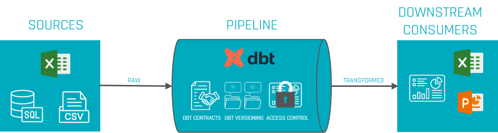
Figure 1: Data contracts act as a safeguard across the entire data pipeline.
Imagine this scenario: A data team has a pipeline to load customer data into a warehouse, and the marketing team relies on it for campaigns. So the downstream consumer, in this case the marketing team, expects fields like customer_name, but an upstream change renames this field to customer_full_name. The marketing team tries to consume this break without anyone immediately noticing. The result? The query would fail since the renamed field is not known to the downstream team. Without a dbt contract, this kind of schema change slips through and causes these downstream failures. When contracts are implemented, however, such a change would trigger an alert or validation error in the pipeline, catching the discrepancy between expected and actual data and preventing the issue.
Data Contracts – Providing Schema Consistency
Data contracts in dbt are a way to ensure what a model is expected to produce. In other words: a contract defines the exact structure of the output table – including which columns are present, what types of data they are or other structural rules. It’s similar to how API contracts work in software: downstream users can count on a consistent format, and if something breaks that expectation, dbt throws an error or a warning during runtime instead of letting flawed data flow further downstream.
With a contract in place, teams can define:
- Which columns must be present – and block unexpected extras or missing fields.
- The type of data (e.g. strings, integers, timestamps).
- Null rules or other constraints, like if a field is allowed to contain null values or can be unique.
These rules are defined in a separate YAML schema file (not directly in the SQL model). For example, a model called orders might have a contract that lists all required columns and their data types, ensuring that every time the model runs, the structure matches what’s been agreed:
models:
- name: orders
  config:
    contract:
      enforced: true
  columns:
    - name: order_id
      data_type: integer
      constraints:
        - type: not_null
    - name: customer_id
      data_type: integer
    - name: order_date
      data_type: date
Once the variable enforced: true (line 5) is set on a model, dbt will validate the output of the SQL before the model is built. It checks that the result includes exactly the expected columns, in the right data types – no extras, no missing fields, no mismatches. If something does not align, dbt throws an error or warning and stops the process before the issue can affect anything downstream. This gives teams a safety net against accidental changes to a model’s structure – whether that’s someone renaming a column, dropping it, or introducing a mismatch in data types.
From a business perspective, this adds a layer of reliability. Teams working with downstream dashboards, reports, or models can rely on a consistent structure without fear that a seemingly small upstream change will quietly break their work. Take the example of a renamed field in a customer model: with a contract in place, that kind of change would’ve been caught during development or CI (Continuous Integration) – before it ever reached production and disrupted reporting. Data contracts bring the discipline of software development (similar to API interface contracts) into analytics work, helping everyone stay aligned on how the data is structured. That is especially valuable in environments where many teams are working from shared models – a clear contract reduces confusion and avoids broken pipelines.
Not every model needs a contract. It’s good to start with critical, high-impact models (those feeding important dashboards or reports). Applying contracts does add some overhead and rigidity, so dbt’s guidance is to ensure your project is sufficiently mature and the model’s schema is relatively stable before enforcing a contract.
Model Versioning – Managing Change Gracefully
In the previous section it became clear that contracts are able to keep the model’s structure. Even with contracts in place, there are situations where besides the model’s structure, the logic needs to be changed. This could go beyond renaming/removing columns or changes in data types and more into e.g. changing the calculation of columns. On a small team, you could probably just make the change and tell everyone to update their queries. But in a larger organization, that kind of quick shift is risky – one change could break a lot of downstream applications like dashboards or other downstream models.
That’s where model versioning comes in (introduced in dbt v1.5+). Model versions bring structure to model evolution. Instead of forcing immediate changes, versioning allows multiple versions of a model to live side by side, giving teams time to transition.
Here’s how it works:
- Create a new version of the model: You start by creating a new version of the model – normally by just duplicating the file with a _v2 suffix – and make your changes there.
- In the model’s YAML config file, you declare all existing versions and mark which one is currently latest.
- Test the new version: During testing, both versions can be run in production. For testing purposes, consumers can point to a specific version explicitly.
- Promote the new version: Once the adjustments are done, the YAML can be updated to make it the latest one.
- Deprecate and remove the old version: Eventually, the old version is deprecated. You can even set a deprecation_date so it’s clear when it will be removed for good. But to be clear, the deprecation_date is just an indicator/piece of information during runtime, the model won’t be deactivated automatically after the date passes.
This approach helps teams migrate in a controlled way. Instead of breaking queries over night, there’s a shared window where both old and new versions exist. Teams have time to update at their own pace, and model authors don’t need to hold back on necessary improvements. It’s a clean parallel to versioned APIs – the idea being that a dbt model, once shared, is similiar to a public interface others rely on.
By treating models as versioned products, data teams avoid having broken queries and are able to regain control over how changes are introduced. It makes collaboration safer and more sustainable, especially when many teams depend on shared upstream models. Therefore, model versioning brings real change management to the day to day work with data.
Note: Model versioning is a concept meant for mature datasets that have multiple dependents. If your project is small or models change rapidly in early development, you might not need to formally version every change. At smaller scale, it’s often acceptable that downstream analyses update in lockstep with model changes. But as you “scale up” the number of models, consumers, or even adopt a data mesh approach with multiple projects, versioning becomes indispensable for stability.
Access Control – Modularizing and Securing Your Models
The third pillar of dbt governance is access control for models. In complex organizations, it’s possible that not every data model is meant to be used everywhere by everyone. Some models are intermediate or meant for a specific team, while others are data products meant for wider consumption. To define what data is accessible for who (ref() function), dbt now allows access levels for each model.
To enable this, dbt introduces the concept of groups and access modifiers:
- Groups: Models can be organized into groups and assign each group an owner. Groups are essentially labels for a set of models that share a logical theme or ownership. This helps turn implicit relationships into explicit boundaries – leading to a clearer model ownership.
- Access modifiers: Each model can be marked as private , protected , or public to indicate its accessibility to other models.
- Private: only other models in the same group can reference it. It’s hidden from the rest of the project.
- Protected: (default) any model within the same project can reference it, but models in other projects cannot. This is how models behaved historically in dbt – accessible project-wide but not exposed to the outside by default.
- Public: any model, even in other projects (or installed packages), can reference it. This explicitly marks the model as part of a public interface for cross-project use.
By default, models are considered protected for backward compatibility. Using groups and access modifiers together, you can make certain models truly private to a specific team while safely sharing others as needed. For example, a finance team’s intermediate calculation model might be tagged private to finance, so only finance models can use it. If a marketing model tried to ref(‘finance_model’) that was private, dbt would throw an error during parsing, blocking the unauthorized dependency. Meanwhile, a carefully designed model of “Customers” might be marked public so that it can be referenced by models in any project across the company.
Why is this valuable?
It enforces modularity and ownership. Teams can develop models without fear that another team will depend on their internal logic. It prevents the problem, that anything can depend on anything, which becomes hard to manage. Instead, only well defined public models become the integration points between different groups or projects. This kind of access governance improves security (sensitive data can be kept in private models) and maintainability, since changes to a private model won’t ripple out beyond its group.
Governance vs. User Permissions: It’s important to differentiate between model access as described above and user-level permissions. The features that was discussed is about design-time and run-time control of model dependencies in dbt projects. In practice, this is used in conjunction with your data warehouse’s security (and dbt Cloud’s user roles) to ensure only the right people or tools can run or query these models. Model governance is about structuring the project for safe collaboration; it complements (but does not replace) standard data access controls.
Conclusion – Toward Reliable and Scalable Data Projects
In summary, dbt’s governance capabilities like contracts, versioning, and access control provide a framework for reliable, scalable data transformation workflows. They bring proven software engineering principles into the analytics engineering realm:
- Data contracts ensure that upstream changes don’t unknowingly break downstream models/consumers by enforcing schemas and data integrity rules at build time.
- Model versioning treats important datasets as stable interfaces, allowing teams to implement improvements without sudden disruptions – enabling change with graceful deprecation instead of chaos.
- Access control (with groups and private/protected/public models) modularizes your project, so teams can work peacefully within their domain while providing clear interfaces and preventing unintended coupling between projects.
Adopting these practices means fewer hotfixes caused by broken pipelines. As one blog put it, when scaling up dbt or moving towards a multi-team data mesh, these governance features become non-negotiable – they let you treat your data models “like products: stable, predictable, and version-controlled”. In short, they help you scale with confidence.
Finally, it’s important that governance features should be introduced thoughtfully. It’s possible to overengineer too early – adding contracts or strict version control to models that are still rapidly evolving may slow the process down. The best approach is to apply these tools to the most critical and stable parts of your data model, and expand as the project needs grow.