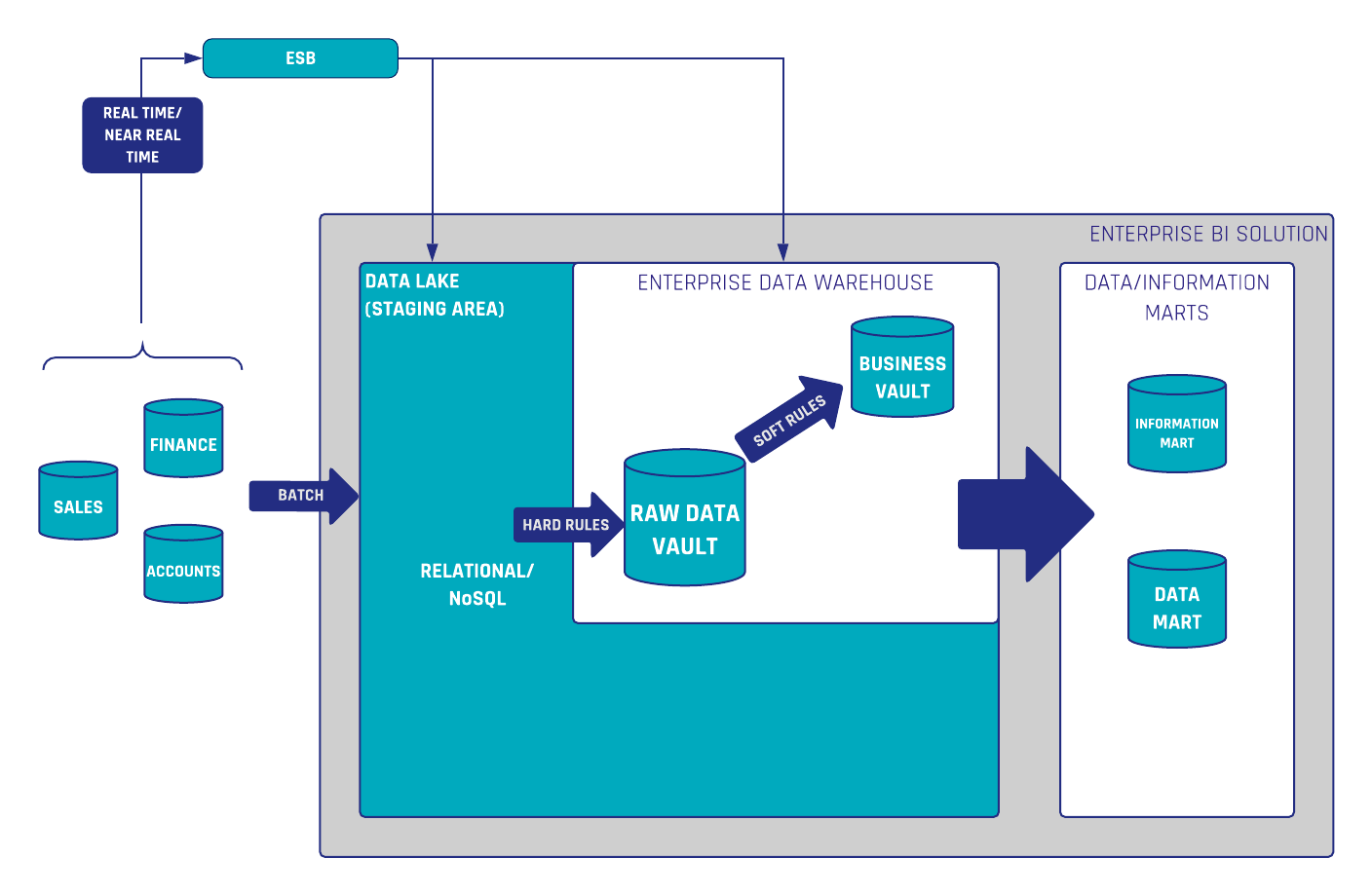
search
0

Data Vault 2.0’s Inventor Offers Unprecedented On-Site Access

To all those that have been a part of the Scalefree journey up until this point,

We’d first and foremost like to thank you for all the contributions you have made in helping us build Scalefree into the firm it is today. All of your contributions and business have allowed us to create a success story beyond what was first imagined and for that we offer our gratitude.

That said, a recent development here at Scalefree has presented the company with the opportunity to offer unprecedented, on-site access to the man that helped make all of this possible, the inventor of Data Vault 2.0, Dan Linstedt.

Though before diving into the unique opportunity that presents you, a little about how we got here.

Continue Reading

Data Vault Use Cases Beyond Classical Reporting – Part 1

Data Cleansing with Data Vault 2.0

Enterprise Data Warehouses with Data Vault 2.0

While Enterprise Data Warehouses (EDWs) are traditionally used for reporting and dashboarding, with Data Vault, their true potential lies far beyond these basic applications. Data Vault 2.0 introduces unparalleled flexibility and scalability, enabling organizations to unlock new use cases such as data cleansing, operational process automation, and predictive analytics. This article explores how Data Vault 2.0 empowers businesses to apply centralized data cleansing rules, enhance data quality at its source, and embrace Total Quality Management (TQM). By leveraging the full capabilities of their EDWs, organizations can move beyond simple analytics to create sustainable, agile, and impactful data strategies.

Going beyond standard reporting with Data Vault 2.0

Reporting and dashboarding have become the standards in business when it comes to identifying KPIs and other measurements. As such, Enterprise Data Warehouses have emerged to support the reporting process. Though, due to the large quantity and variety of data, a demand has developed for a method of utilizing this existing data in a manner in which it can add additional business value towards a company’s needs. Data Vault 2.0 offers a wide range of methods to provide decision support beyond standard reporting as well as critical information regarding the future. To see for yourself, join us as we present different approaches and solutions as to fully leverage the potential of your data.

Watch webinar recording

Flexibility and Scalability

To put it simply, an Enterprise Data Warehouse (EDW) collects data from your company’s internal as well as external data sources, to be used for simple reporting and dashboarding purposes. Often, some analytical transformations are applied to that data as to create the reports and dashboards in a way that is both more useful and valuable. That said, there exist additional valuable use cases which are often missed by organizations when building a data warehouse. The truth being, EDWs can access untapped potential beyond simply reporting statistics of the past. To enable these opportunities, Data Vault brings a high grade of flexibility and scalability to make this possible in an agile manner.

Data Vault Use Cases

To begin, the data warehouse is often used to collect data as well as preprocess the information for reporting and dashboarding purposes only. When only utilizing this single aspect of an EDW, users are missing opportunities to take advantage of their data by limiting the EDW to such basic use cases.

A whole variety of use cases can be realized by using the data warehouse, e.g. to optimize and automate operational processes, predict the future, push data back to operational systems as a new input or to trigger events outside the data warehouse, to simply explore but a few new opportunities available.

Continue Reading

Requirements and Templates for Hashing

Solutions

REQUIREMENTS FOR HASHING

Traditional data warehouses often use sequence numbers to identify records in other tables.

By using sequences, this method comes with some drawbacks. One of the biggest drawbacks is performance. Since the sequence numbers are generated by a generator, this step presents a bottleneck. In addition sequence numbers are generated in the data warehouse instead of loading them before.

This solution provides a template and the requirements round about hashing.

ACCESS THE SOLUTION

What to Consider for Naming Conventions in Data Warehousing – Part 1

Naming conventions - Letter cases

Naming Conventions in Data Warehousing

An initial decision of critical importance within Data Vault development relates to the definition of naming conventions for database objects. As part of the development standardization, these conventions are mandatory to maintain a well-structured and consistent Data Vault model. It is important to note that proper naming conventions boost the usability of the data warehouse, not only for solution developers but also for power users within data exploration.

Throughout this article, we will present the most vital considerations within our standard book, the process of defining naming conventions.

Naming Convention Documentation

It is one aspect to simply define naming conventions utilized within the development of your data warehouse, but it is completely another to establish consistency to create defined naming conventions that are to become standards. That said, it is a good practice to document a guideline for naming Data Warehouse objects. To that end, the next sections will discuss several considerations to take into account when defining the naming conventions for a data warehouse solution.

Naming Conventions: Letter case

There are several options when it comes to considering letter cases for names: all uppercase, all lowercase, Camel Case, and Pascal Case. Though the variances may be slight, each option does have its own advantages and disadvantages regarding legibility as well as type-ability, to briefly touch upon the differences.

Ultimately, the decision regarding letter case falls to the decision of which database management system is used as some, such as PostgreSQL, support case-sensitive object name that requires the use of quoted names. Therefore, users often prefer the lower-case by default in PostgreSQL as having lower-cased object names can reduce the amount of code that is to be generated while simultaneously improving the usability for ad-hoc queries by power users. Nevertheless, it is imperative to maintain one consistent letter case for both entity and column names.

Naming conventions - Letter cases
Figure 1: Naming Convention - Letter Case

Naming Conventions: Usage of underscores “_”, hyphens “-”

To improve readability, word separators like underscores “_” or, depending on use cases, hyphens/dashes “-” are desirable. However, it is important to remember that in many systems, hyphens are interpreted as minus signs. That said, hyphens are commonly used in XML or JSON data format though they can be easily replaced by underscores, should the latter be used as separators.

Naming Conventions: Abbreviation, acronyms

Some systems enforce character limits on object names, e.g. Oracle 12.1 and below only allows for a maximum object name length of 30 bytes. Therefore, abbreviations and acronyms may be taken into consideration during the object naming process, even though they can often lead to misinterpretation. To combat this, it is suggested to compile a document containing a list of the abbreviations being used with a detailed description of their meanings. However, to limit any possible confusion avoid excessive use of abbreviations and acronyms.

In logical models, it is advisable, that object names are as self-explanatory as possible, i.e. most words should be fully spelled out, except common abbreviations for longer words such as “dept” for “department” or “org” for “organization”. However, abbreviations and acronyms are typically used in physical models, to keep object names short.

Naming Conventions: Singular vs. plural object names

It is a common practice to utilize nouns or noun phrases, in their singular form, as object names. This is done to avoid the necessity of dealing with irregular pluralization in English, e.g. man/men, person/people, which would unnecessarily add a whole new level of complexity within the data model.

Naming Conventions: Prefix vs. Suffix

Whether objects are named using prefixes or suffixes, is not of much importance within the development. That said, internally at Scalefree, we prefer table names with suffixes such as “customer_h”, and “transaction_l” instead of utilizing prefixes. The advantage of this method is that, given most database tools sort tables alphabetically, all tables, that are related to a business object, will be grouped. For example, all contact hubs, satellites, and links that have names beginning with “contact_…” will, therefore, be found together in the browser. This supports data exploration by power users and developers.

Naming conventions - prefix
Figure 2: Naming Convention - Prefix

Nevertheless, prefixes can be meaningful within some use cases, e.g. using prefix in layer schema names helps keeping them neatly listed together in the database browser.

Naming conventions - Schema
Figure 3: Naming Convention - Schemas

Conclusion

Naming conventions are partially a matter of personal preference and organizational guidelines. Regardless, the more systematically consistent the naming conventions become when defined, the more benefits will ultimately be seen within the development and implementation of your Data Vault solution. To illustrate this point, we encourage Data Vault development teams to write and implement a simple SQL function that inspects the entire database while checking for naming convention inconsistencies. This further ensures that standards are being followed.

Interested in how we standardize naming conventions here at Scalefree? In an upcoming article, we will share several concrete suggestions for naming conventions, most of which both our customers and our team regularly utilize internally.

Now let’s open this up for discussion in the comment box below: How do you implement naming conventions within your Data Vault development? What conventions do you follow?

Data Security Concepts in Data Vault 2.0

Solutions

Data Security Concepts

The focal point of our discussion revolves around critical aspects such as security controls, access controls, and the definition of identities. The primary objective of this solution is to safeguard data assets effectively. The approach taken is typically centered on securing data at both the row/document level and the attribute level.

In terms of security controls, the emphasis is on implementing measures that ensure the confidentiality, integrity, and availability of data. Access controls play a pivotal role in governing who can interact with specific data assets, limiting access to authorized individuals or roles. Defining identities involves establishing clear parameters for users and entities accessing the data, contributing to a robust security framework.

In summary, this Data Vault solution prioritizes a comprehensive approach to data security, addressing concerns at different levels to fortify the protection of valuable data assets.

ACCESS THE SOLUTION

Exemplary Naming Conventions in Data Vault 2.0

Solutions

Naming Conventions

Data Vault modeling is a powerful approach that introduces a multitude of entities to the database. To enhance usability and facilitate effective development, it is highly advisable to implement clear and consistent naming conventions. These conventions play a vital role in grouping entities by concept and conveying crucial information to developers, including the data source, rate of change, privacy levels, security considerations, and more.

Introducing a well-thought-out naming convention not only simplifies the development process but also contributes to a more organized and comprehensible database structure. It acts as a guide for developers, offering insights into the nature and characteristics of each entity.

Conversely, the absence of a naming convention poses challenges in identifying related tables within Data Vault models. This lack of structure can lead to confusion, making it harder for developers to discern the relationships and purpose of different entities.

In conclusion, the implementation of naming conventions is fundamental for the success of Data Vault modeling solutions. It promotes clarity, efficiency, and a systematic approach to database development.

ACCESS THE SOLUTION

Bridge Tables 101: Why They Are Useful

Bridge Tables Screenshot of Connections

What Are Bridge Tables?

Bridge tables are special entities within the Data Vault that leverage query performance on the way out of the Data Vault. These entities are placed between the Data Vault and the Information Delivery Layer and are necessary for instances in which many joins and aggregations on the Raw Data Vault are executed, causing performance issues.

This often happens when designing the virtualized fact tables in the information and data marts. Thus, to produce the required granularity in the fact tables without increasing the query time, bridge tables come into play. Bridge tables belong to the Business Vault and have the purpose of improving performance, similar in manner to the PIT table which was discussed in a prior newsletter.

As a means to achieve its goals, bridge tables materialize the grain shift that is often required within the information delivery process. Though, before we dig deeper into the specifics of using bridge tables for performance tuning, it is important to first define granularities within a data warehouse.

Grain Definitions in Data Warehousing

The grain within a dimensional model is the level of detail available of each table. Thus, the grain of a fact table is defined by the number of related dimensions. Basically, there are three different types of granularities for fact entities within a dimensional model. Continue Reading

Alternative to the Driving Key Implementation in Data Vault 2.0

Driving Key Source Table

Alternative to the Driving Key

There is a special case when a part of the hub references stored in a link can change without describing a different relation. This has a great impact on the link satellites. Furthermore, back in 2017 we introduced the link structure with an example of a Data Vault model in the banking industry. We showed how the model looks like when a link represents either a relationship or a transaction between two business objects. A link can also connect more than two hubs. What is the alternative to the Driving Key implementation in Data Vault 2.0?

The Driving Key

A relation or transaction is often identified by a combination of business keys in one source system. In Data Vault 2.0 this is modelled as a normal link connecting multiple hubs each containing a business key. A link contains also its own hash key, which is calculated over the combination of all parents’ business keys. So when the link connects four hubs and one business key changes, the new record will show a new link hash key. There is a problem when four business keys describe the relation, but only three of them identify it as unique. We can not identify the business object by using only the hash key of the link. The problem is not a modeling error, but we have to identify the correct record in the related satellite when query the data. In Data Vault 2.0 this is called a driving key. It is a consistent key in the relationship and often the primary key in the source system.

The following tables demonstrate the relationship between an employee and a department from a source system.

Driving Key Source Table
Table 1: employee-department relationship

The following Data Vault model can be derived from this source structure.

Driving Key in a Data Vault Model
Figure 1: Data Vault model

The link table “Empl_Dep” is derived from the table “Employee” in the source system. The Driving Key in this example is the Employee_Number as it is the primary key in the source table, and an employee can work in only one department at the same time. This means, the true Driving Key “lives” in the satellite of the employee. If the department of an employee switches, there is no additional record in the employee’s satellite table, but a new one in the link table, which is legitimate.

Driving Key in a Data Vault Model
Table 2: link data

To query the most recent delta you have to query it from the link table, grouped by the driving key.

To sum up you will always have a new link hash key when a business key changes in a relation. The challenge is to identify the driving key, which is a unique business key (or a combination of business keys) for the relationship between the connected hubs. Sometimes you would have to add an additional attribute to get a unique identifier.

Both present an issue for power users with access to the Data Vault model. Without naming conventions there is a risk that a group by statement is performed on more attributes than just the driving key which would lead to unexpected and incorrect aggregate values – even though the data itself is correctly modeled.

When dealing with relationship data there is a better solution available than the driving key: we typically prefer to model such data as a non-historized link and insert technical counter-transactions to the data when a hub reference changes.

In the case of a modified record in the source, we insert two records to the non-historized links: one for the new version of the modified record in the source and one for the old version that still exists in the target (non-historized link) but needs to be countered now – the technical counter record. To distinguish the records from the source and the counter transactions a new column is inserted, often called “Counter”.

The standard value for this counter attribute is 1 for records from the source and -1 for the technical counter transactions. Important: We do not perform any update statements, we still insert only the new counter records. When querying the measures from the link you just multiply the measures with the counter value.

Driving Key in a Data Vault Model
Table 3: LinkConnection with counter attribute

The table 3 shows a link with a counter attribute. When a record changes in the source system it is inserted with the original value and a counter value of -1 in the link table of the data warehouse. For the changed value there is a new link hash key which is also calculated over the descriptive attribute ‘Salary’. The counter value of the new record is 1.

Conclusion

Because identifying the driving key of a relation can be a problem in some situations you can use an alternative solution to avoid the driving key. All changes and deletes are tracked using a counter attribute in the non-historized link table. It stores also the descriptive attributes and the link hash key is calculated over all attributes.

Test Strategies for Data Vault 2.0 based EDW

Solutions

Test Strategies

Testing is very important for data warehouse systems to make them work correctly and efficiently. In unit testing, each component is separately tested.

By testing business logic using unit tests, there is an issue with available tools for unit testing in data warehouses.

This solution describes test strategies for enterprise data warehouse solutions based on Data Vault 2.0.

ACCESS THE SOLUTION

How to Implement Insert Only in Data Vault 2.0?

End dating satellites in Data Vault 2.0 for insert only architecture

Insert Only in Data Vault 2.0

Skilled modeling is important to harness the full potential of Data Vault 2.0. To get the most out of the system due to scalability and performance, it also has to be built on an architecture which is completely insert only. On the way into the Data Vault, all update operations can be eliminated and loading processes simplified.

The common implementation in Data Vault 2.0

In the common loading patterns, there are two important technical timestamps in Data Vault 2.0. The first is the load date timestamp (LDTS). This timestamp does not represent a business date that comes from the source system. Instead, it provides information about when the data was first loaded into the data warehouse, usually the staging area.

Therefore, it is completely different from the various business dates that come from the source systems including a business meaning. For this reason, it must be generated for a whole batch-loading process. Business dates, for example, validation dates, are stored in effectivity satellites, which are mostly found connected with link entities. They provide information about the relationship of business objects with begin and end date of a relationship.

The second technical timestamp is the load end date timestamp (LEDTS). Like the LDTS, the LEDTS is system-generated and occurs in satellite entities only. As those satellites are delta-driven, there is always one record that represents the most recent delta. The value of the LEDTS on those records is usually ‘9999-12-31’ (end of time) or NULL. The following figure shows the whole end-dating process that comes with the usage of the LEDTS attribute. It is executed after the loading process of the satellite (not in the loading process):

End dating satellites in Data Vault 2.0 for insert only architecture
Figure 1: End dating process for satellites

The figure shows that we have to update the satellite with the new LEDTS value which costs performance. As mentioned in the beginning we want to remove the LEDTS updates to get more performance with a 100% insert-only Data Vault 2.0 architecture.

At this point, a typical question is how to query the most recent delta in a satellite when we don’t have the LEDTS anymore. Using max(LDTS)? For sure not.

The advantage of PIT tables in Data Vault 2.0

The answer is to use window functions to load your point in time (PIT) tables. We covered the topic PIT tables with an example from the insurance industry in our newsletter from October 2018. The purpose of PIT tables is to improve the query performance by eliminating outer joins and allow inner joins with equi join conditions for performance reasons. We highly recommend building a PIT table as the better alternative to the LEDTS. The PIT table is built using window functions to find the most recent delta in the satellite. Once it is created with snapshots of the current data, we don’t have to query on the LDTS with BETWEEN conditions. The temporal history is stored as snapshots and can be queried with equi join conditions on the Hash Key and the LDTS to the related satellites. Due to the fact that the PIT tables grow, it is recommended to create partitions on the snapshot date. At the end, the (visualized) Information Mart dimensions can be easily queried directly from the PIT table and the related satellites.

By using window functions on the Hash Key (partition) and the LDTS (order) you can identify the most recent delta, which is dynamically calculated. There are some window functions that can be used for finding the most recent delta. The following table shows some examples for window functions.

Window function in Data Vault 2.0 for insert only architecture
Table 1: Examples of window functions

A reason for the existence of the LEDTS in Data Vault is that many databases in the early 21st century were not supporting window functions or were not fast enough.

As already mentioned in the previous newsletter of October 2018, the purpose of PIT tables is to allow inner joins with equi join conditions. But they are also the key to get to an insert-only implementation of Data Vault 2.0, which allows more efficient loading processes.

Conclusion

Implementing an insert-only architecture in Data Vault 2.0 enhances scalability and performance by eliminating update operations during data loading. This approach simplifies the loading process and ensures that all data changes are captured as new records, preserving historical accuracy. By utilizing Point-in-Time (PIT) tables, organizations can efficiently query the most recent data without relying on end-dating techniques, further streamlining data retrieval and analysis.

How to Use Point in Time Tables (PIT) in the Insurance Industry?

Introduction to point in time tables

Point in Time Tables

Point in time tables are useful when querying data from the Raw Vault that has multiple satellites on a hub or a link:

Introduction to point in time tables
Figure 1: Data Vault model including PIT (logical)

About Point In Time Tables Tables

In the above example, there are multiple satellites on the hub Customer and link included in the diagram. This is a very common situation for data warehouse solutions because they integrate data from multiple source systems. However, this situation increases the complexity when querying the data out of the Raw Data Vault. The problem arises because the changes to the business objects stored in the source systems don’t happen at the same time. Instead, a business object, such as a customer (an assured person), is updated in one of the many source systems at a given time, then updated in another system at another time, etc. Note that the Point-in-time table (PIT) is already attached to the hub, as indicated by the ribbon.

Changes came in at various times, not related to each other. Most updates would be added when insurance is concluded, but they did not affect all operational systems at the same time. As a consequence, the change did not affect all satellites. Instead, it affected only the satellite that was supposed to cover the change (which is an advantage).

When building a data mart from this raw data, querying the customer data on a given date becomes complicated: the query should return the customer data as it was active according to the data warehouse delta process on the selected date. It requires outer join queries with complex time range handling involved to achieve this goal. With more than three satellites on a hub or link, this becomes complicated and slow. The better approach is to use equal-join queries for retrieving the data from the Raw Data Vault. To achieve this, a special entity type is used in Data Vault 2.0 modeling: point in time tables (PIT). This entity is introduced to a Data Vault 2.0 model whenever the query performance is too low for a given hub or link and surrounding satellites.

Point in time tables
Figure 2: PIT table structure

Because the data in a PIT table is system-computed and does not originate from a source system, the data is not to be audited and not in the Raw Vault, so the structure can be modified to include computed columns.

Point in time tables serve two purposes:

Simplify the combination of multiple deltas at different “point in time”

A PIT table creates snapshots of data for dates specified by the data consumers upstream. For example, it is often usual to report the current state of data each day. To accommodate these requirements, the PIT table includes the date and time of the snapshot, in combination with the business key, as a unique key of the entity (a hashed key including these two attributes, named CustomerKey in Figure 2). For each of these combinations, the PIT table contains the load dates and the corresponding hash keys from each satellite that correspond best with the snapshot date.

Reduce the complexity of joins for performance reasons with point in time tables

The point in time table is like an index used by the query and provides information about the active satellite entries per snapshot date. The goal is to materialize as much of the join logic as possible and end up with an inner join with equi-join conditions only. This join type is the most performant version of joining on most (if not all) relational database servers. In order to maximize the performance of the PIT table while maintaining low storage requirements, only one ghost record is required in each satellite used by the point in time table. This ghost record is used when no record is active in the referenced satellite and serves as the unknown or NULL case. By using the ghost record, it is possible to avoid NULL checks in general, because the join condition will always point to an active record in the satellite table: either an actual record that is active at the given snapshot date or the ghost record.

Example of Point in time tables
Table 1: Example of PIT table

The table above (Table 1) shows an assured person with frozen data states, one from the 8th, and one from the 9th of October 2018. On the 8th there was no record for this customer in the legal expenses insurance satellite. For that reason both the hash key and the load date timestamp are NULL. For better query performance, these NULL values are pointed to the ghost record in the related satellite table to avoid searching for a record which not exist.

When customer data must be deleted for one business only and PII information is used as Business Key, just the Link entry and the descriptive attributes in the specific Satellite have to be deleted. The activity history is still available, can be used for analytical reasons, and is not traceable to the customer itself. The additional advantage of this “business split” is when only one business is affected in case of deleting customer data, i.e. each business comes from different subsidiaries, and only the car insurance data must be deleted. Furthermore, keep in mind that deleting the Business Key only (and keeping the Hash Key) does not result in GDPR compliance (and does not meet the Data Vault 2.0 standard anyway as the Business Key is used in link tables). The Hash Key in Data Vault 2.0 is not used to encrypt data but for performance reasons. The key in the Links and the business-driven Hubs, as we are talking about, can not be calculated back as it is a complete surrogate key. As soon as the customer wants to be deleted completely as he/she is no longer a customer in any of your business, you delete the record from the main Hub as well.

Otherwise, if there is no additional artificial key for the customer, after deleting PII data, you can not tie your data back to an object (an anchor point), which makes them (in many cases) useless.

Conclusion

The purposes of point in time tables are to improve the query performance by eliminating outer joins and allowing inner joins with equi join conditions (best performance). Additionally, point in time tables enhance partitioning and enable full scalability of star schemas (which should be completely virtualized) on top of the Data Vault. Furthermore, end users don’t have to join through all satellite tables, but join just one table for one business object which reduces the query complexity for ad-hoc queries.

Close Menu