Why Data Vault 2.0?

This blog article discusses some features where Data Vault 2.0 can shine and why you should use it. As a database developer, administrator or user, you probably have already heard of Data Vault. But with an existing database solution in mind, you might come to the question of why you should use Data Vault in your enterprise data warehouse. 

Reason 1: Supporting multiple source systems and frequently changing relationships

Data Vault 2.0 provides the most benefits when your data comes from many source systems or has constantly changing relationships. 

Data Vault 2.0 works well for multi-source systems or those that have constantly changing relationships.

The reason why it works well for these systems is its ability to make adding attributes simple. If there is a change to one source system, that change does not need to show up within all source systems. Similarly, you can limit the number of places changes are made, as attributes are stored separately from structural data in satellites.

Additionally, it is easier to account for new and changing relationships by closing off one link and creating another. You don’t have to change the historical data to account for a new relationship or update an existing schema. You only need to account for the changes going forward. This brings enormous flexibility and scalability into your enterprise data warehouse.

Reason 2: Easily track and audit your data with Data Vault 2.0

In a modern data environment, the data runs through various different stops. To still provide continuous data quality, it must always be clear where data has come from. 

Figure 1: Data Lineage

Given the need to be able to easily track and audit data, Data Vault has made it easier to do so. It does so by inherently enabling auditing, as load times and record sources are required for every row. It also tracks all historical changes as satellites, including the load time as part of the primary key.
When an attribute is updated, a new record is created.
All of this auditing enables you to easily provide auditability for both regulatory and data governance purposes. And because you store all of your history, you can access data from any point in time.

Reason 3: Load data from multiple source systems more quickly with Data Vault 2.0

Data Vault enables quicker data loading simply because a number of tables can be loaded at the same time in parallel. The model decreases dependencies between tables during the load process and simplifies the ingestion process by leveraging inserts only, which load quicker than upserts or merges. This also leads to less complexity.

Conclusion

Data Vault 2.0 is designed to integrate data from several source systems and may over perform in some situations.

In summary, if you have a small to medium-sized analytics requirement, with a small team of architects, designers, and engineers delivering a solution with data sourced from a few systems, then Data Vault may be inappropriate for your need.

If, however, you have a large project with many source systems leading to an enormous data integration challenge, then Data Vault can potentially add massive value to the project.

Multi-Active Satellites in Data Vault 2.0

In our first post about multi-active satellites, we briefly explained different implementations that can be used to solve multi-activity. Now, we’re going to go into more detail regarding the advantages and disadvantages of these approaches having delta checks on or off.

Short Summary of Multi-Active Satellites

Multi-active satellites allow you to implement multi-active records per business key in Data Vault 2.0. To illustrate the need for the solution, let’s look at the common occurrence of a source system that doesn’t provide the needed metadata such as when working with XML files.

One solution to the above is to create a multi-active satellite by adding a subsequence number per business key. This accounts for any instance in which there is no multi-active attribute delivered by the source itself. Regarding phone numbers, this information could be a tag for a business, home, or mobile phone number. Another possibility is to create an extra hub for the multi-active attribute. However, since it doesn’t present a real business object, the first solution can be more effective.

Delta Check OFF

There are two ways to insert new records into a multi-active satellite – having delta checks active or inactive. With delta checks turned off, all records of a business key are inserted into the satellite from your source delivery.

The advantage of that is that loads are faster and have a consistent load date timestamp to the parent hash key, independent of the multi-active attribute.

Later on, it simplifies the query based on the multi-active data (see Figure 1). As a critical drawback, the ingested amount of data can increase strongly if full data loads are received.

In this case, you should partition your data by the load date timestamp. 

Figure 1: Joining records using one PIT-table when having one LDTS for all active records per key.

Delta Check ON

To reduce the amount of data simply use delta checks. Doing so, you match the incoming data with the latest LDTS per hash key.
Note that a useful function to leverage the delta check is LISTAGG(). This function transforms values from a group of rows into a list of values. As a result, you are able to create a hash difference of multi-active attributes per business key (see figure 2).

Figure 2 – Multi-row hash difference using the LISTAGG()-function

If new data arrives, it can be compared by the multi-row hash difference. Using it, a high proportion of data can be ignored. When a delta is detected, all records are inserted per hash key even if the content of the data for only one subsequence is changed. The result is that you get a consistent load date timestamp per hash key. Additionally, a delta is going to be noticed when the order of records changes as well. This approach is a trade-off to reduce the amount of records while still having a consistent load date timestamp per hash key so that only one PIT table is necessary.

Using Type Codes

Another method to address multi-activity is to use types of the attributes, granted they exist, as explained in the previous post.
If you have type codes in place, you’re able to compare row by row and load only this specific data. But consequently, you get different LDTS per multi-active attribute. Using PIT-tables in the business vault, you’ll therefore need an extra multi-active PIT-table. This scenario is shown in figure 3.

Figure 3 – The need for an MA-PIT having different LDTS of active records per key

If you can pivot the multi-active column into multiple columns, one column per characteristic, you won’t need to consider any of the above advantages or disadvantages. In this case, you turn the satellite into a standard satellite. Related to our example with the phone numbers, you would create a couple of new columns per phone type.
This solution is applicable if you can be certain that the characteristics of the phone types will not change in the future. Otherwise, you will have to reengineer your process to catch all the data you have delivered!

Conclusion

In our second post regarding  multi-active satellites, we explored the backgrounds behind the different methods. You can use this information to implement your own multi-active solution depending on your present data.
Though, note that it’s often recommended limiting the loading data. For this purpose, the LISTAGG()-function becomes useful. Using a solution with potentially different LDST, remember to consider them when querying the data.

Effort Estimation in Data Vault 2.0 Projects

In Data Vault 2.0 projects, we recommend estimating the effort by applying a Function Point Analysis (FPA), but there are many options available when choosing a method to estimate the necessary effort within agile IT projects. In this article, you will learn why FPA is a good choice and why you should consider using this method in your own Data Vault 2.0 projects.

Good Old Planning Poker for Effort Estimation

Probably the best known method for estimating work in agile projects is Planning Poker. Within the process, so-called story points, based upon the Fibonacci sequence (0, 0.5, 1, 2, 3, 5, 8, 13, 20, 40 and 100), are used to estimate the effort of a given task. To begin the process, the entire development team sits together as each member simultaneously assigns story points to each user story that they feel are appropriate. If the story points match, the final estimate is made. Alternatively, if a consensus cannot be reached the effort is discussed until a decision is made. 

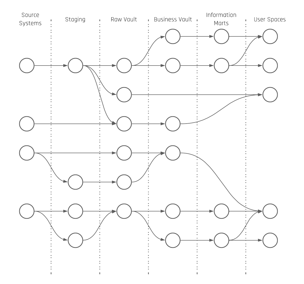
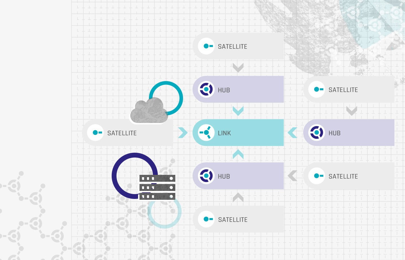
However, it’s important to note that this technique involves a lot of effort as a result of either too many tasks or too many team members.  So the question is: Does Planning Poker work for Data Vault projects? The short answer is “it makes little sense”. Since in Data Vault 2.0 the functional requirements are broken down into small items, there are numerous tasks that all have to be discussed and evaluated. In addition, the subtasks in Data Vault 2.0 are standardized artifacts, such as Hub, Link, and Satellite. In principle, these artifacts always represent the same effort.

Why does Function Point Analysis suit it so well?

This is where FPA comes into play and the reason why it is widely used in agile software projects. The idea is that software consists of the following characteristics, which represent the Function Point Types:

• External inputs (EI) → data entering the system
• External outputs (EO), external inquiries EQ → data leaving the system one way or another
• Internal logical files (ILF) → data manufactured and stored within the system
• External interface files (EIF) → data maintained outside the system but necessary to perform the task

With FPA, you break the functionality into smaller items for better analysis. As mentioned, this is already done in Data Vault 2.0 projects due to the standardized artifacts. This is the reason why FPA is very suitable for Data Vault projects.

How to apply FPA in Data Vault 2.0

Hence, to make good use of FPA in the Data Vault 2.0 methodology, the functional characteristics of software, external inputs, external outputs, external inquiries, internal logical files, and external interface files, must be adapted to reflect Data Vault projects. The following functional characteristics of data warehouses built with Data Vault are defined as:

• Stage load (EI)
• Hub load (ILF)
• Link load (ILF)
• Satellite load (ILF)
• Dimension load (ILF)
• Fact load (ILF)
• Report build (EO)

Please note that there are also other functional components that can be defined, like Business Vault entities, Point-in-time tables, and so on. Once you have defined these components, you should create a table that maps them to function points. Function points are used to quantify the amount of business functionality an element provides to a user. In general, it is recommended to add a complexity factor first:

Complexity Factor	Person Hours per Function Point
Easy	0.1
Moderate	0.2
Difficult	0.7

Then use the complexity factors and the assigned function points per component to calculate the estimated hours needed to add the respective functionality. Here is a short example of how the mapping table could look like for you:

Component	Complexity Factor	Estimated Function Points	Estimated Total Hours
Hub Load	Easy	2	0.2
Dimension Load	Difficult	3	2.1
Report Build	Difficult	5	3.5

The goal of estimation is to standardize the development of operational information systems by making the effort more predictable. This is due to the fact that when you use a systematic approach to estimate the needed effort to add components, it is possible to compare the estimated values with the actual values once the functionality is delivered. When both values are compared, your team can learn from these previous estimates and improve their future estimates by adjusting the function points per component. Also, keep in mind that your developers will gain experience over time or might lose experience due to replacement.

Conclusion

I hope this first glimpse into FPA helps you understand the basic value it can provide your team in Data Vault 2.0 projects. You can have a more in-depth look at how to apply FPA in Data Vault 2.0 projects by reading the book “Building a Scalable Data Warehouse with Data Vault 2.0” by Michael Olschimke and Dan Lindstedt.